Learning Algorithm Evaluation Introduction Overfitting

Learning Algorithm Evaluation

Introduction

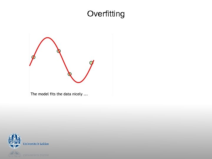Overfitting

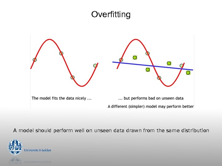Overfitting A model should perform well on unseen data drawn from the same distribution

Evaluation Rule #1 Never evaluate on training data

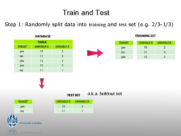Train and Test Step 1: Randomly split data into training and test set (e. g. 2/3 -1/3) a. k. a. holdout set

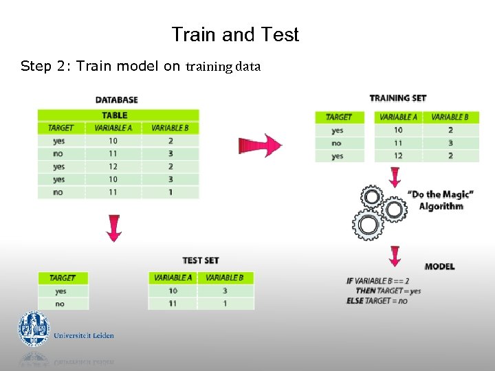Train and Test Step 2: Train model on training data

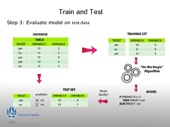Train and Test Step 3: Evaluate model on test data

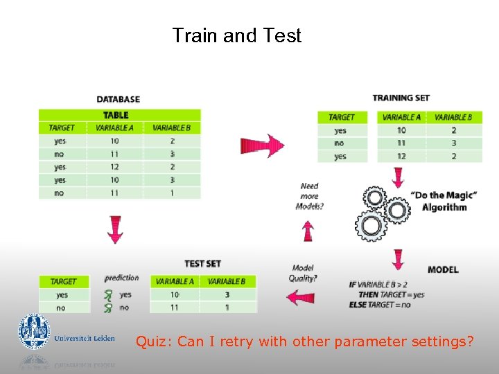Train and Test Quiz: Can I retry with other parameter settings?

Evaluation Rule #1 Never evaluate on training data Rule #2 Never train on test data (that includes parameter setting or feature selection)

Test data leakage g Never use test data to create the classifier g g Separating train/test can be tricky: e. g. social network Proper procedure uses three sets g g g training set: train models validation set: optimize algorithm parameters test set: evaluate final model

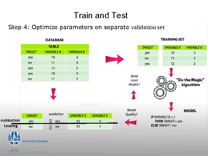Train and Test Step 4: Optimize parameters on separate validation set validation testing

Making the most of the data g g Once evaluation is complete, all the data can be used to build the final classifier Trade-off: performance evaluation accuracy g g More training data, better model (but returns diminish) More test data, more accurate error estimate

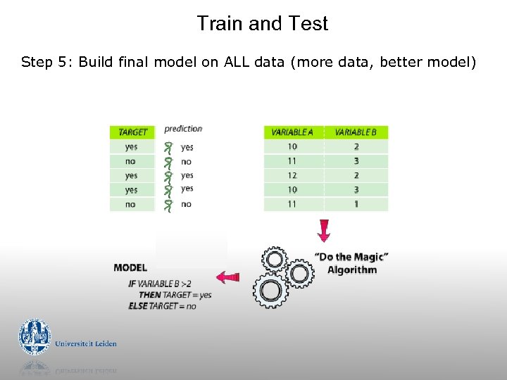Train and Test Step 5: Build final model on ALL data (more data, better model)

Cross-Validation

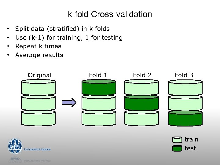k-fold Cross-validation • • Split data (stratified) in k folds Use (k-1) for training, 1 for testing Repeat k times Average results Original Fold 1 Fold 2 Fold 3 train test

Cross-validation g Standard method: g g Stratified ten-fold cross-validation 10? Enough to reduce sampling bias g Experimentally determined

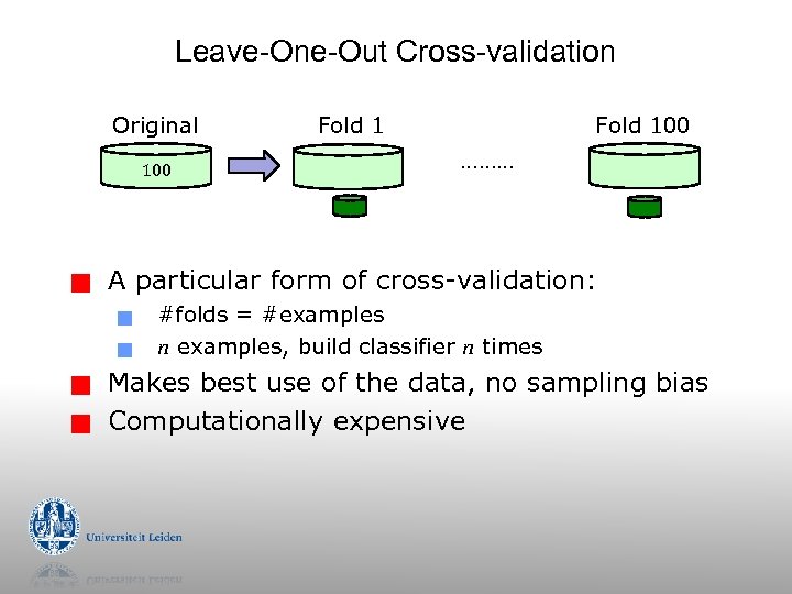Leave-One-Out Cross-validation Original 100 g g g Fold 100 ……… A particular form of cross-validation: g g Fold 1 #folds = #examples n examples, build classifier n times Makes best use of the data, no sampling bias Computationally expensive

ROC Analysis

ROC Analysis g g g Stands for “Receiver Operating Characteristic” From signal processing: trade-off between hit rate and false alarm rate over noisy channel Compute FPR, TPR and plot them in ROC space Every classifier is a point in ROC space For probabilistic algorithms g Collect many points by varying prediction threshold

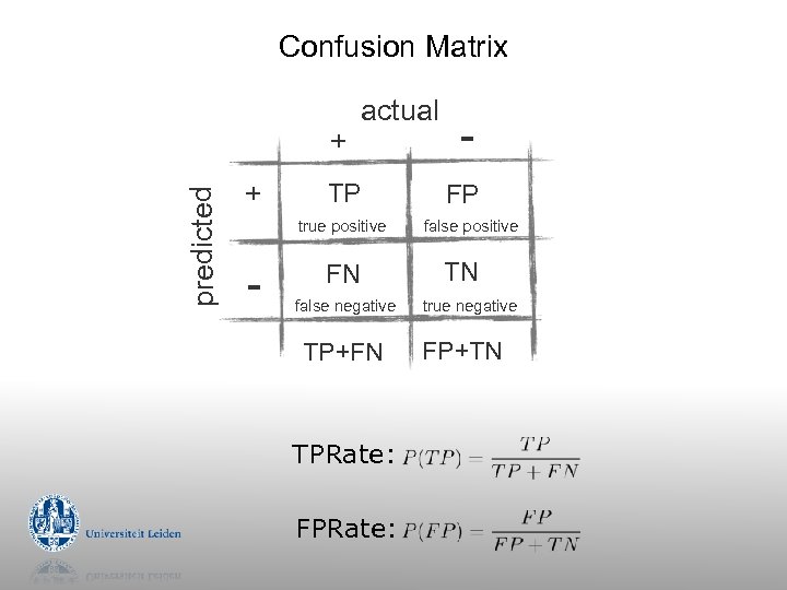Confusion Matrix predicted + + actual TP true positive - FN false negative TP+FN TPRate: FPRate: FP false positive TN true negative FP+TN

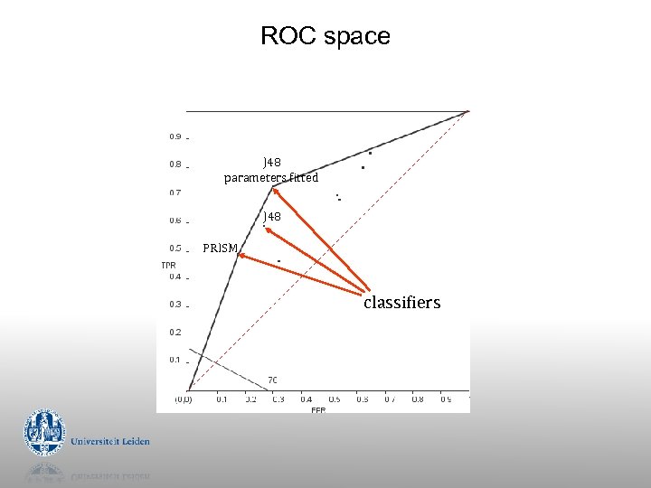ROC space J 48 parameters fitted J 48 PRISM classifiers

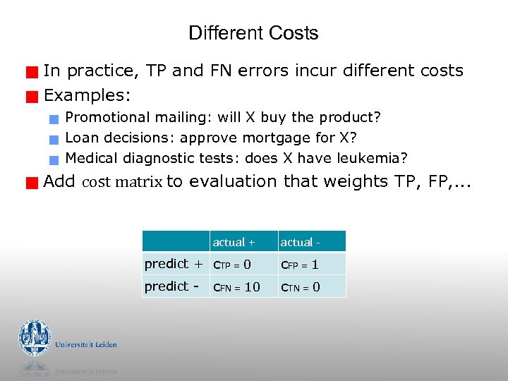Different Costs In practice, TP and FN errors incur different costs g Examples: g g g Promotional mailing: will X buy the product? Loan decisions: approve mortgage for X? Medical diagnostic tests: does X have leukemia? Add cost matrix to evaluation that weights TP, FP, . . . actual + predict + c. TP = 0 predict - c. FN = 10 actual - c. FP = 1 c. TN = 0

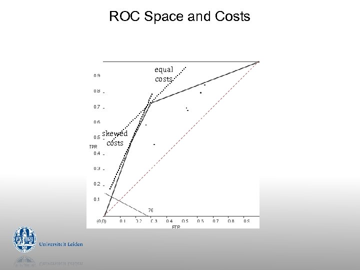ROC Space and Costs equal costs skewed costs

Statistical Significance

Comparing data mining schemes g Which of two learning algorithms performs better? g Note: this is domain dependent! Obvious way: compare 10 -fold CV estimates g Problem: variance in estimate g g g Variance can be reduced using repeated CV However, we still don’t know whether results are reliable

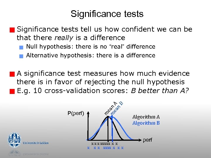Significance tests g Significance tests tell us how confident we can be that there really is a difference g g Null hypothesis: there is no “real” difference Alternative hypothesis: there is a difference A significance test measures how much evidence there is in favor of rejecting the null hypothesis g E. g. 10 cross-validation scores: B better than A? P(perf) m e m an ea A n B g x xxxxx x x xxxx x Algorithm A Algorithm B perf

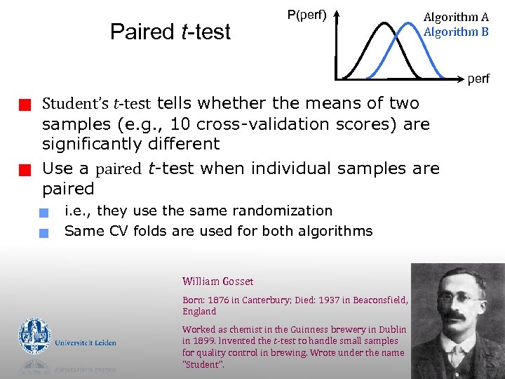Paired t-test P(perf) Algorithm A Algorithm B perf g g Student’s t-test tells whether the means of two samples (e. g. , 10 cross-validation scores) are significantly different Use a paired t-test when individual samples are paired g g i. e. , they use the same randomization Same CV folds are used for both algorithms William Gosset Born: 1876 in Canterbury; Died: 1937 in Beaconsfield, England Worked as chemist in the Guinness brewery in Dublin in 1899. Invented the t-test to handle small samples for quality control in brewing. Wrote under the name "Student".

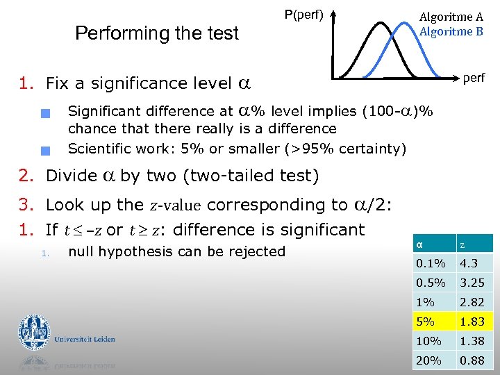P(perf) Performing the test 1. Fix a significance level g g perf Significant difference at % level implies (100 - )% chance that there really is a difference Scientific work: 5% or smaller (>95% certainty) 2. Divide by two (two-tailed test) 3. Look up the z-value corresponding to /2: 1. If t –z or t z: difference is significant 1. Algoritme A Algoritme B null hypothesis can be rejected α z 0. 1% 4. 3 0. 5% 3. 25 1% 2. 82 5% 1. 83 10% 1. 38 20% 0. 88