LC Technology Manufacturing Systems Quality Management

LC Technology Manufacturing Systems

Quality Management – Pareto Analysis Pinpoints problems through the identification and separation of the ‘vital few’ problems from the trivial many. Vilifredo Pareto: concluded that 80% of the problems with any process are due to 20% of the causes.

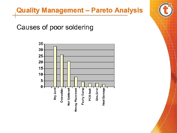Quality Management – Pareto Analysis Causes of poor soldering

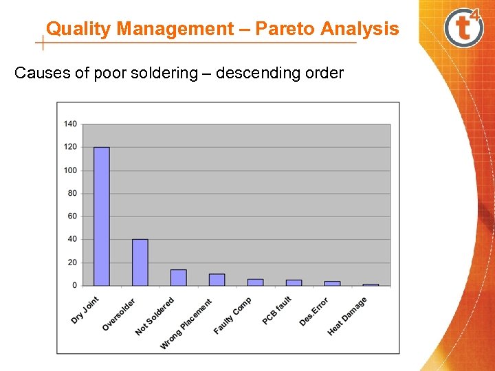Quality Management – Pareto Analysis Causes of poor soldering – descending order

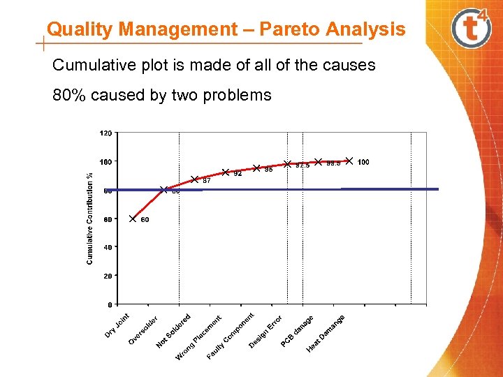Quality Management – Pareto Analysis Cumulative plot is made of all of the causes 80% caused by two problems

Statistical Process Control • Statistical procedure to verify quality • Check manufacturing process is working correctly →Inspect and measure manufacturing process →Varying from target – corrective action taken • Prevents poor quality before it occurs

Statistical Process Control When? Manufacturing large quantities of items • Euro coins • Computers • Cars etc. Why? • Impractical to measure each item made • Machine/equipment/human error How? • Measure a small proportion of the produced items (sample) • Use X-bar and R Charts to see if process is in control • Conclude the quality characteristics of the whole process

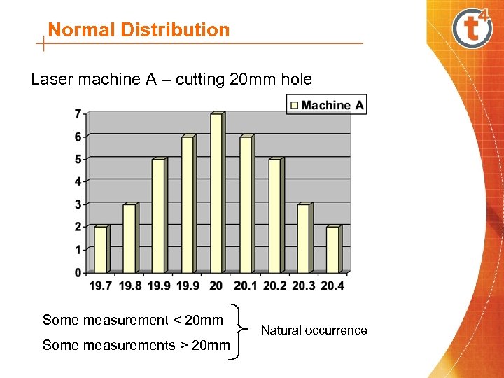Normal Distribution Laser machine A – cutting 20 mm hole Some measurement < 20 mm Some measurements > 20 mm Natural occurrence

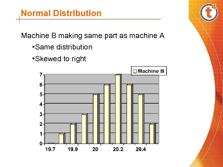Normal Distribution Machine B making same part as machine A • Same distribution • Skewed to right

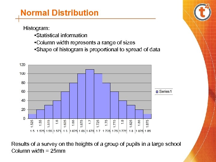Normal Distribution Histogram: • Statistical information • Column width represents a range of sizes • Shape of histogram is proportional to spread of data Results of a survey on the heights of a group of pupils in a large school Column width = 25 mm

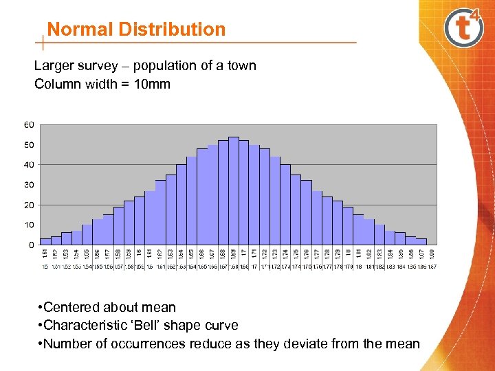Normal Distribution Larger survey – population of a town Column width = 10 mm • Centered about mean • Characteristic ‘Bell’ shape curve • Number of occurrences reduce as they deviate from the mean

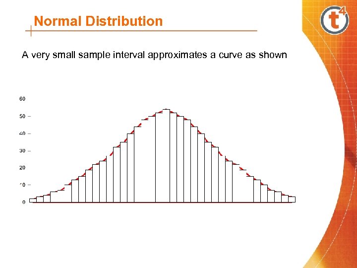Normal Distribution A very small sample interval approximates a curve as shown

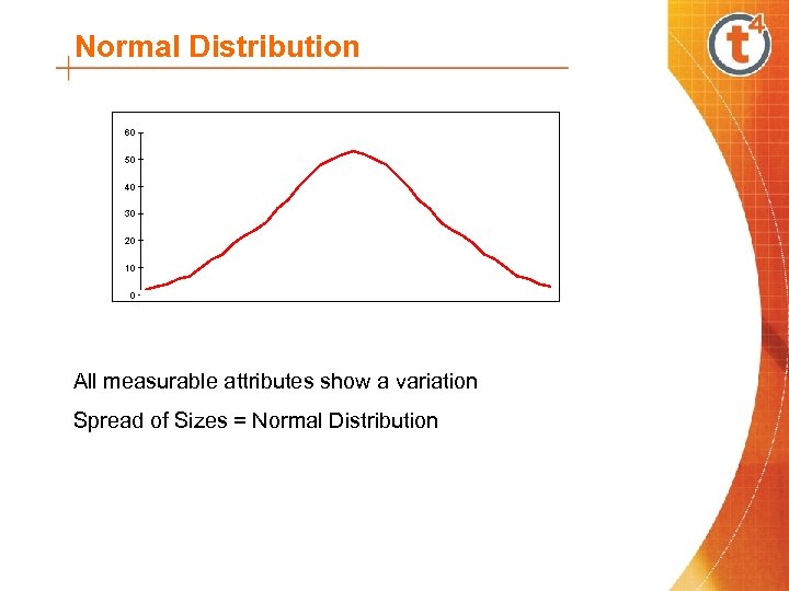Normal Distribution 60 50 40 30 20 10 0 All measurable attributes show a variation Spread of Sizes = Normal Distribution

Normal Distribution • The spread or ‘width’ of the curve has a precise mathematical meaning - Variance • The greater the variance the wider the curve • Defined by a parameter called the standard deviation

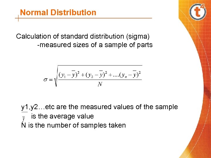Normal Distribution Calculation of standard distribution (sigma) -measured sizes of a sample of parts y 1, y 2…etc are the measured values of the sample is the average value N is the number of samples taken

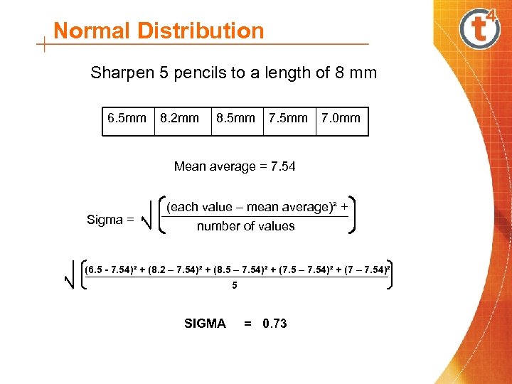Normal Distribution Sharpen 5 pencils to a length of 8 mm 6. 5 mm 8. 2 mm 8. 5 mm 7. 0 mm Mean average = 7. 54 Sigma = (each value – mean average)² + number of values (6. 5 - 7. 54)² + (8. 2 – 7. 54)² + (8. 5 – 7. 54)² + (7 – 7. 54)² 5 SIGMA = 0. 73

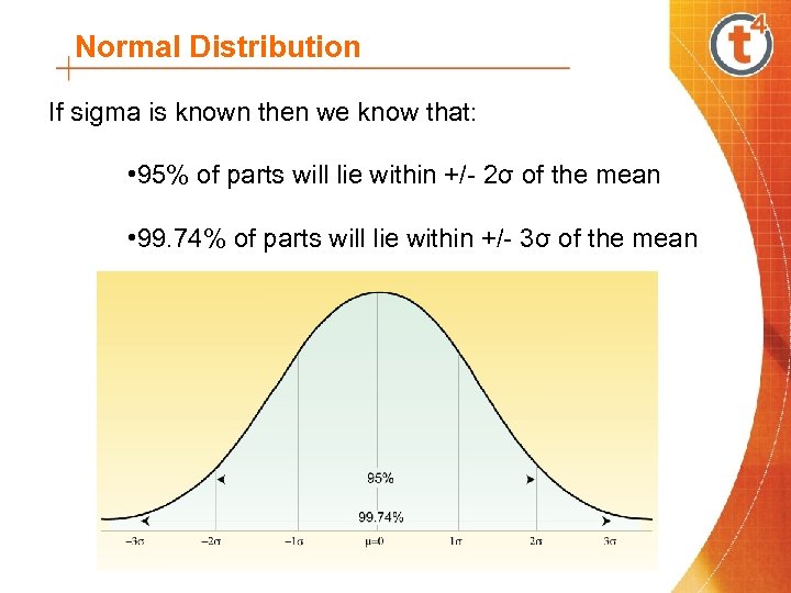Normal Distribution If sigma is known then we know that: • 95% of parts will lie within +/- 2σ of the mean • 99. 74% of parts will lie within +/- 3σ of the mean

Control Charts • Used to establish the control limits for a process • Used to monitor the process to show when it is out of control 1. X-bar Chart (Mean Charts) 2. R Charts (Range Charts)

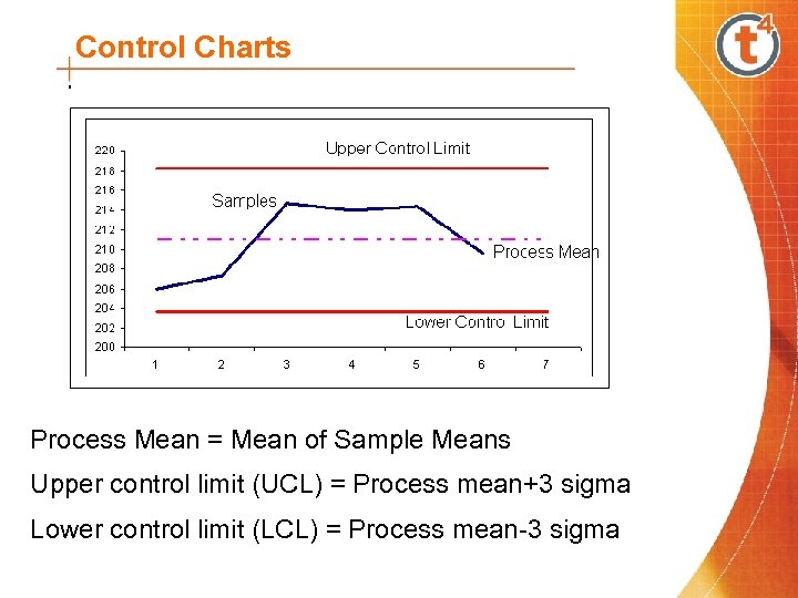Control Charts Process Mean = Mean of Sample Means Upper control limit (UCL) = Process mean+3 sigma Lower control limit (LCL) = Process mean-3 sigma

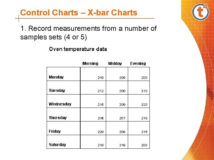Control Charts – X-bar Charts 1. Record measurements from a number of samples sets (4 or 5)

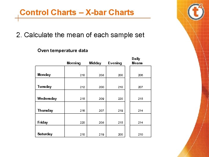Control Charts – X-bar Charts 2. Calculate the mean of each sample set Oven temperature data Morning Midday Evening Daily Means Monday 210 208 200 206 Tuesday 212 200 210 207 Wednesday 215 209 220 215 Thursday 216 207 219 214 Friday 220 208 215 214 Saturday 210 219 200 210

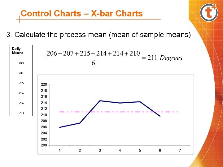Control Charts – X-bar Charts 3. Calculate the process mean (mean of sample means) Daily Means 206 207 215 214 210

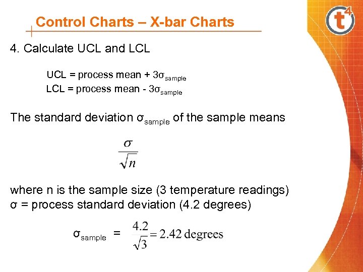Control Charts – X-bar Charts 4. Calculate UCL and LCL UCL = process mean + 3σsample LCL = process mean - 3σsample The standard deviation σsample of the sample means where n is the sample size (3 temperature readings) σ = process standard deviation (4. 2 degrees) σsample =

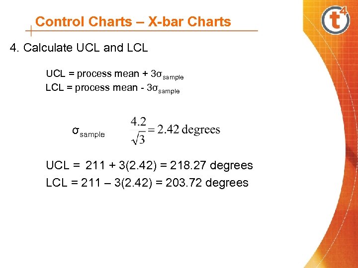Control Charts – X-bar Charts 4. Calculate UCL and LCL UCL = process mean + 3σsample LCL = process mean - 3σsample UCL = 211 + 3(2. 42) = 218. 27 degrees LCL = 211 – 3(2. 42) = 203. 72 degrees

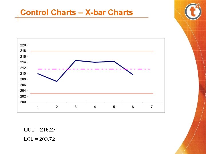Control Charts – X-bar Charts UCL = 218. 27 LCL = 203. 72

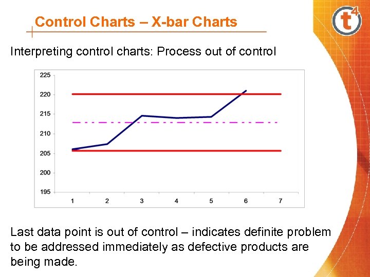Control Charts – X-bar Charts Interpreting control charts: Process out of control Last data point is out of control – indicates definite problem to be addressed immediately as defective products are being made.

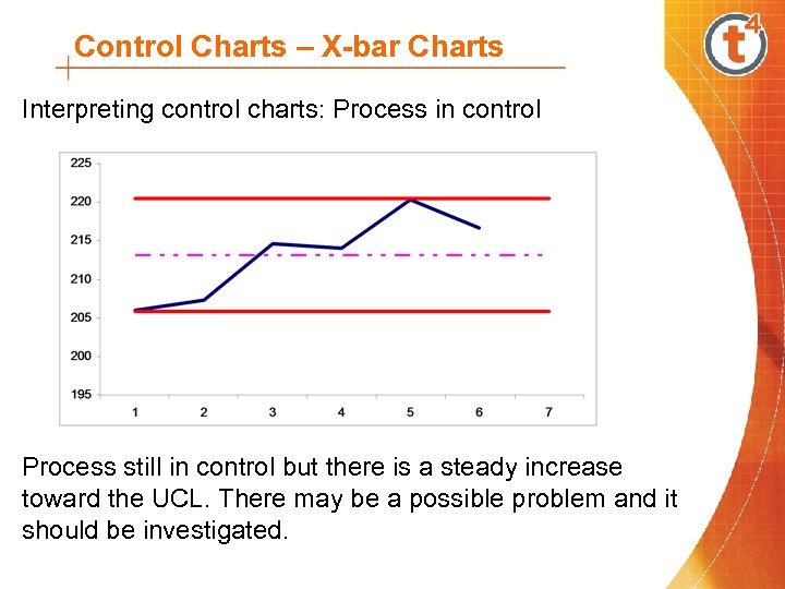Control Charts – X-bar Charts Interpreting control charts: Process in control Process still in control but there is a steady increase toward the UCL. There may be a possible problem and it should be investigated.

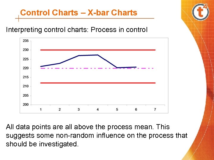Control Charts – X-bar Charts Interpreting control charts: Process in control All data points are all above the process mean. This suggests some non-random influence on the process that should be investigated.

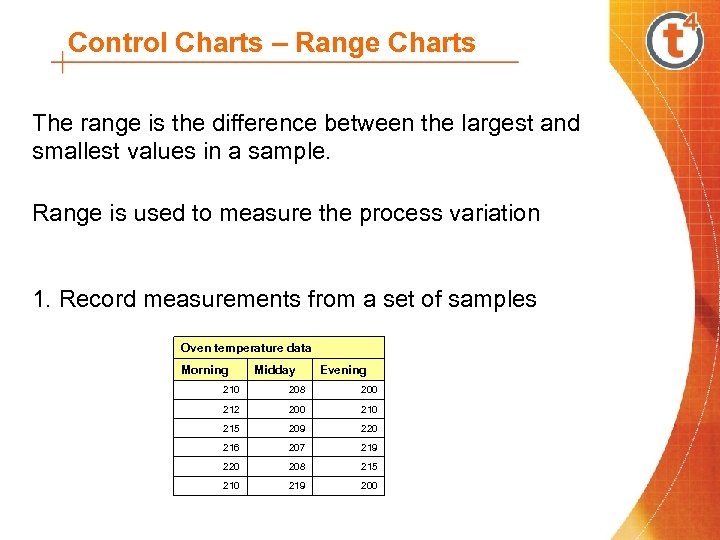Control Charts – Range Charts The range is the difference between the largest and smallest values in a sample. Range is used to measure the process variation 1. Record measurements from a set of samples Oven temperature data Morning Midday Evening 210 208 200 212 200 215 209 220 216 207 219 220 208 215 210 219 200

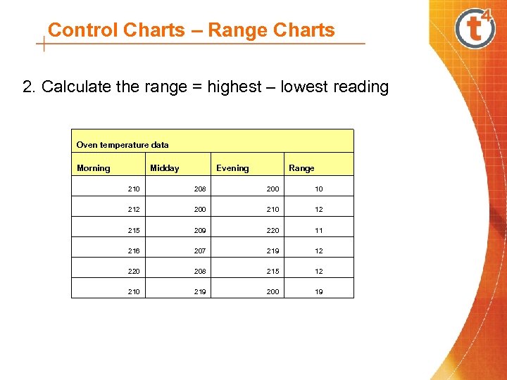Control Charts – Range Charts 2. Calculate the range = highest – lowest reading Oven temperature data Morning Midday Evening Range 210 208 200 10 212 200 210 12 215 209 220 11 216 207 219 12 220 208 215 12 210 219 200 19

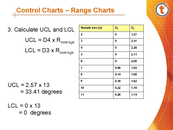Control Charts – Range Charts LCL = 0 x 13 = 0 degrees 0 3. 27 3 0 2. 57 4 0 2. 28 5 0 2. 11 0 2. 00 0. 08 1. 92 8 UCL = 2. 57 x 13 = 33. 41 degrees D 4 7 LCL = D 3 x Raverage D 3 6 UCL = D 4 x Raverage Sample size (n) 2 3. Calculate UCL and LCL 0. 14 1. 86 9 0. 18 1. 82 10 0. 22 1. 78 11 0. 26 1. 74

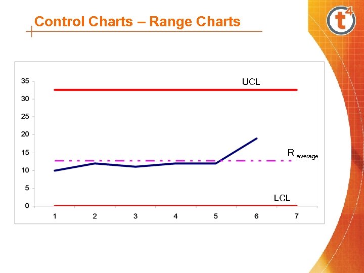Control Charts – Range Charts UCL R average LCL

Process Capability Matches the natural variation in a process to the size requirements (tolerance) imposed by the design Filling a box with washers: • exact number not in all boxes • upper limit set • lower limit set

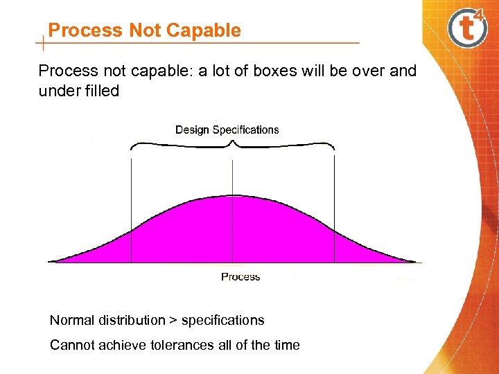Process Not Capable Process not capable: a lot of boxes will be over and under filled Normal distribution > specifications Cannot achieve tolerances all of the time

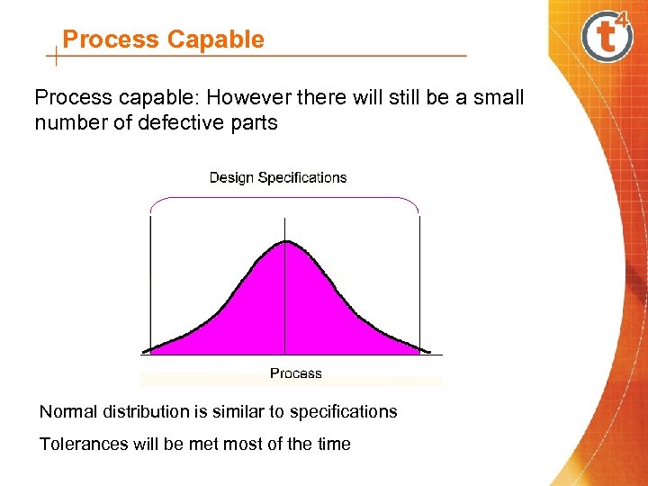Process Capable Process capable: However there will still be a small number of defective parts Normal distribution is similar to specifications Tolerances will be met most of the time

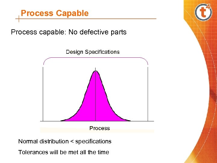Process Capable Process capable: No defective parts Normal distribution < specifications Tolerances will be met all the time

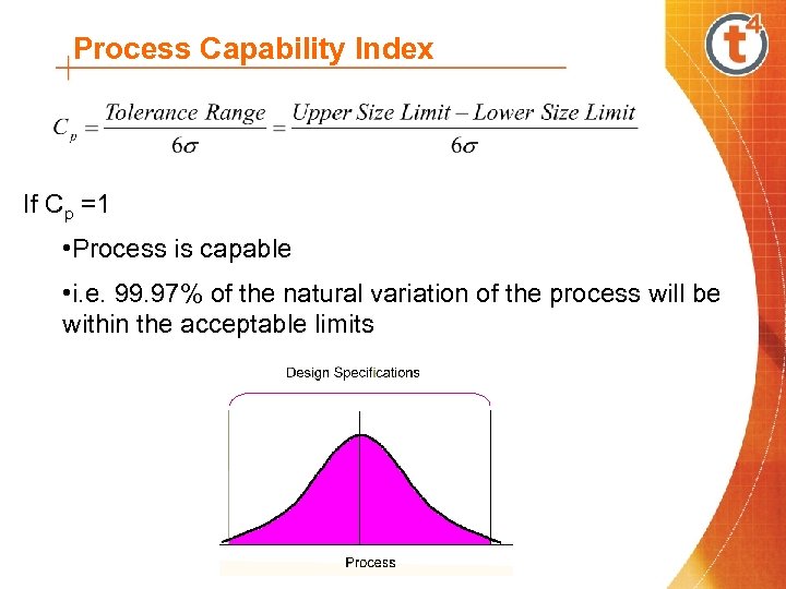Process Capability Index If Cp =1 • Process is capable • i. e. 99. 97% of the natural variation of the process will be within the acceptable limits

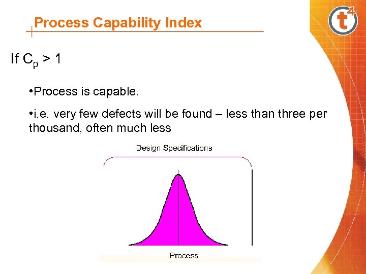Process Capability Index If Cp > 1 • Process is capable. • i. e. very few defects will be found – less than three per thousand, often much less

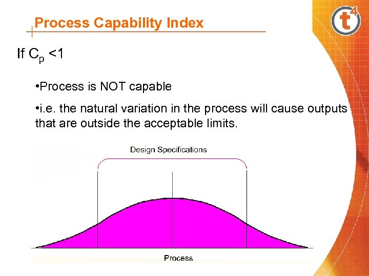Process Capability Index If Cp <1 • Process is NOT capable • i. e. the natural variation in the process will cause outputs that are outside the acceptable limits.

Statistical Process Control Is doing things right 99% of the time good enough? 13 major accidents at Heathrow Airport every 2 days 5000 incorrect surgical procedures per week ……………… Pharmaceutical company producing 1 000 tablets a week, 99% quality would mean 10 000 tablets would be defective! Process of maintaining high quality standards is called : Quality Assurance Modern manufacturing companies often aim for a target of only 3 in a million defective parts. The term six sigma is used to describe quality at this level

Sampling Size of Sample? Sufficient to allow accurate assessment of process • More – does not improve accuracy • Less – reduced confidence in result

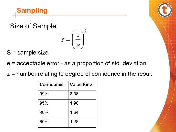Sampling Size of Sample S = sample size e = acceptable error - as a proportion of std. deviation z = number relating to degree of confidence in the result Confidence Value for z 99% 2. 58 95% 1. 96 90% 1. 64 80% 1. 28

Sampling Example – find mean value for weight of a packet of sugar • with a confidence of 95% • acceptable error of 10% • Weight of packet of sugar = 1000 g • Process standard deviation = 10 g

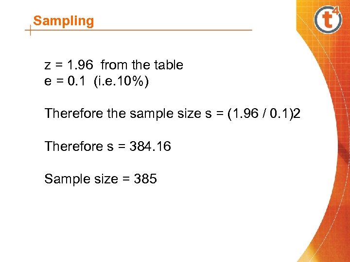Sampling z = 1. 96 from the table e = 0. 1 (i. e. 10%) Therefore the sample size s = (1. 96 / 0. 1)2 Therefore s = 384. 16 Sample size = 385

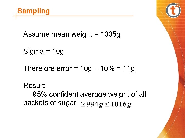Sampling Assume mean weight = 1005 g Sigma = 10 g Therefore error = 10 g + 10% = 11 g Result: 95% confident average weight of all packets of sugar

QC, QA and TQM Quality Control: • emerged during the 1940 s and 1950 s • increase profit and reduce cost by the inspection of product quality. • inspect components after manufacture • reject or rework any defective components Disadvantages: • just detects non-conforming products • does not prevent defects happening • wastage of material and time on scrapped and reworked parts inspection process not foolproof • possibility of non-conforming parts being shipped by mistake

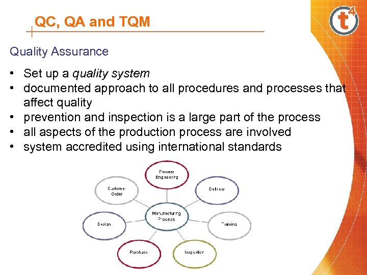QC, QA and TQM Quality Assurance • Set up a quality system • documented approach to all procedures and processes that affect quality • prevention and inspection is a large part of the process • all aspects of the production process are involved • system accredited using international standards

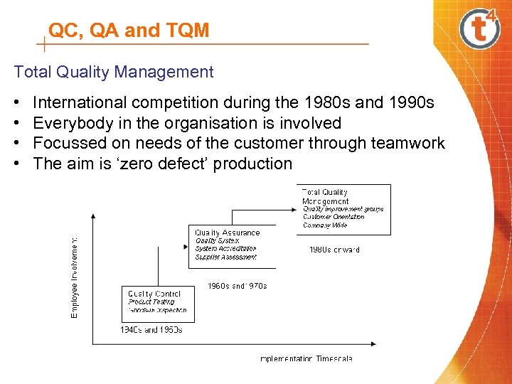QC, QA and TQM Total Quality Management • • International competition during the 1980 s and 1990 s Everybody in the organisation is involved Focussed on needs of the customer through teamwork The aim is ‘zero defect’ production

Just-In-Time Manufacture Modern products – shortened life cycle Manufacturer – pressure for quick response Quick turnaround - hold inventory of stock Holding inventory costs money for storage Inventory items obsolete before use New approach: Just-In-Time Manufacture

Just-In-Time Manufacture Underlying concept: Eliminate waste. Minimum amount: • Materials • Parts • Space • Tools • Time Suppliers are coordinated with manufacturing company.

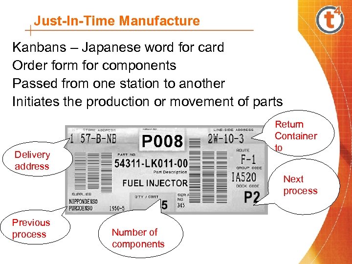Just-In-Time Manufacture Kanbans – Japanese word for card Order form for components Passed from one station to another Initiates the production or movement of parts Return Container to Delivery address Next process Previous process Number of components