Last Time Histograms Binomial Probability Distributions

Last Time • Histograms – Binomial Probability Distributions – Lists of Numbers – Real Data – Excel Computation • Notions of Center – Average of list of numbers – Weighted Average

Administrative Matters Midterm I, coming Tuesday, Feb. 24 • Excel notation to avoid actual calculation – So no computers or calculators • Bring sheet of formulas, etc. • No blue books needed (will just write on my printed version)

Administrative Matters Midterm I, coming Tuesday, Feb. 24 • Material Covered: HW 1 – HW 5 – Note: due Thursday, Feb. 19 – Will ask grader to return Mon. Feb. 23 – Can pickup in my office (Hanes 352) – So this weeks HW not included

Administrative Matters Midterm I, coming Tuesday, Feb. 24 • Extra Office Hours: – Monday, Feb. 23 8: 00 – 9: 00 – Monday, Feb. 23 9: 00 – 10: 00 – Monday, Feb. 23 10: 00 – 11: 00 – Tuesday, Feb. 24 8: 00 – 9: 00 – Tuesday, Feb. 24 9: 00 – 10: 00 – Tuesday, Feb. 24 1: 00 – 2: 00

Administrative Matters Midterm I, coming Tuesday, Feb. 24 • How to study: – Rework HW problems • • Since problems come from there Actually do, not “just look over” In random order (as on exam) Print HW sheets, use as a checklist – Work Practice Exam • Posted in Blackboard “Course Information” Area

Reading In Textbook Approximate Reading for Today’s Material: Pages 277 -282, 34 -43 Approximate Reading for Next Class: Pages 55 -68, 319 -326

Big Picture • Margin of Error • Choose Sample Size Need better prob tools Start with visualizing probability distributions

Big Picture • Margin of Error • Choose Sample Size Need better prob tools Start with visualizing probability distributions, Next exploit constant shape property of Bi

Big Picture Start with visualizing probability distributions, Next exploit constant shape property of Binom’l

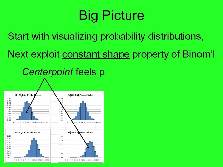
Big Picture Start with visualizing probability distributions, Next exploit constant shape property of Binom’l Centerpoint feels p

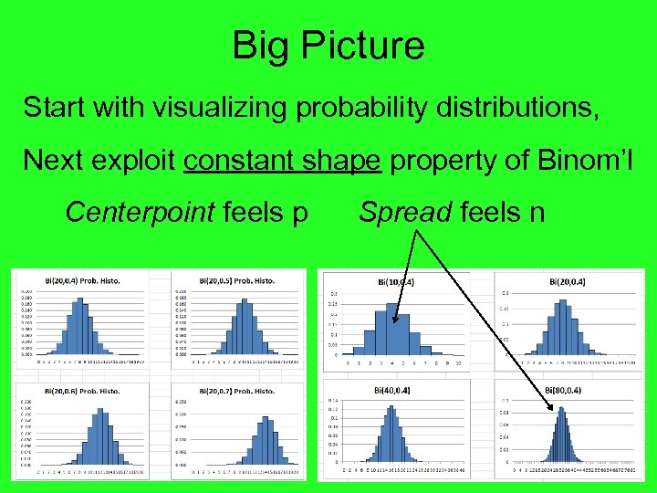
Big Picture Start with visualizing probability distributions, Next exploit constant shape property of Binom’l Centerpoint feels p Spread feels n

Big Picture Start with visualizing probability distributions, Next exploit constant shape property of Binom’l Centerpoint feels p Spread feels n Now quantify these ideas, to put them to work

Notions of Center Will later study “notions of spread”

Notions of Center Textbook: Sections 4. 4 and 1. 2 Recall parallel development: (a) Probability Distributions (b) Lists of Numbers Study 1 st, since easier

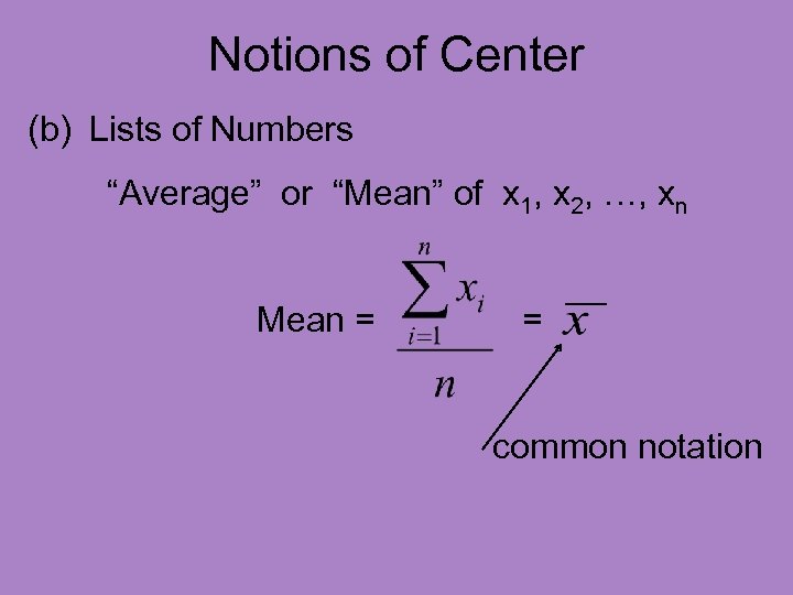
Notions of Center (b) Lists of Numbers “Average” or “Mean” of x 1, x 2, …, xn Mean = = common notation

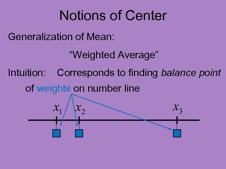
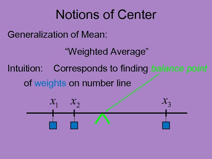
Notions of Center Generalization of Mean: “Weighted Average” Intuition: Corresponds to finding balance point of weights on number line

Notions of Center Textbook: Sections 4. 4 and 1. 2 Recall parallel development: (a) Probability Distributions (b) Lists of Numbers

Notions of Center (a) Probability distributions, f(x) Approach: use connection to lists of numbers

Notions of Center (a) Probability distributions, f(x) Approach: use connection to lists of numbers Recall: think about many repeated draws

Notions of Center (a) Probability distributions, f(x) Approach: use connection to lists of numbers Draw X 1, X 2, …, Xn from f(x)

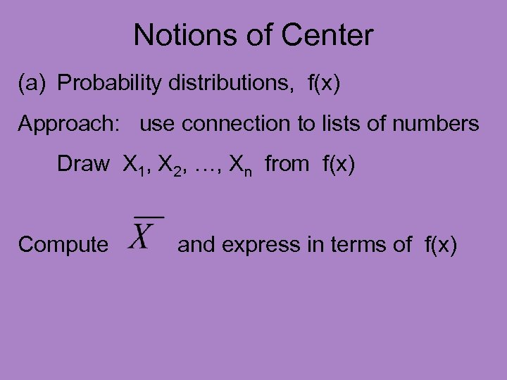
Notions of Center (a) Probability distributions, f(x) Approach: use connection to lists of numbers Draw X 1, X 2, …, Xn from f(x) Compute and express in terms of f(x)

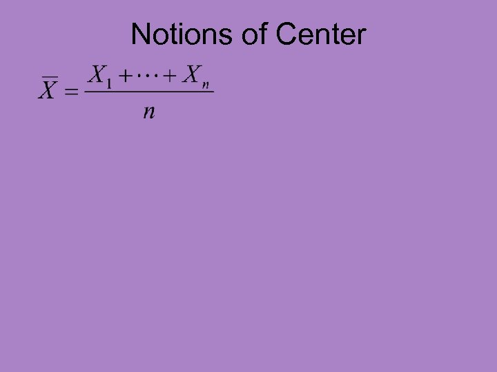
Notions of Center

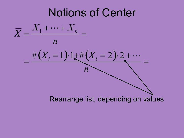
Notions of Center Rearrange list, depending on values

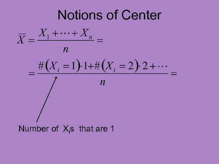
Notions of Center Number of Xis that are 1

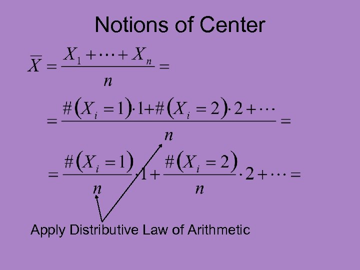
Notions of Center Apply Distributive Law of Arithmetic

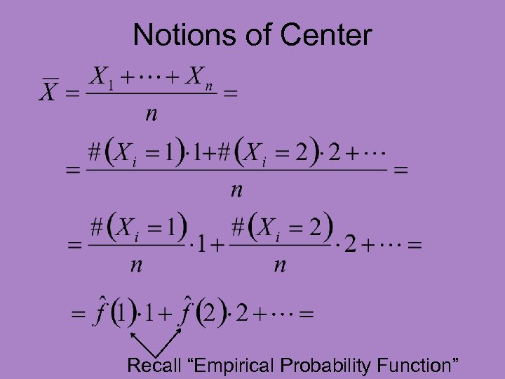
Notions of Center Recall “Empirical Probability Function”

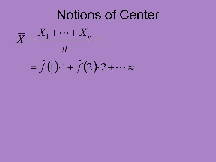
Notions of Center

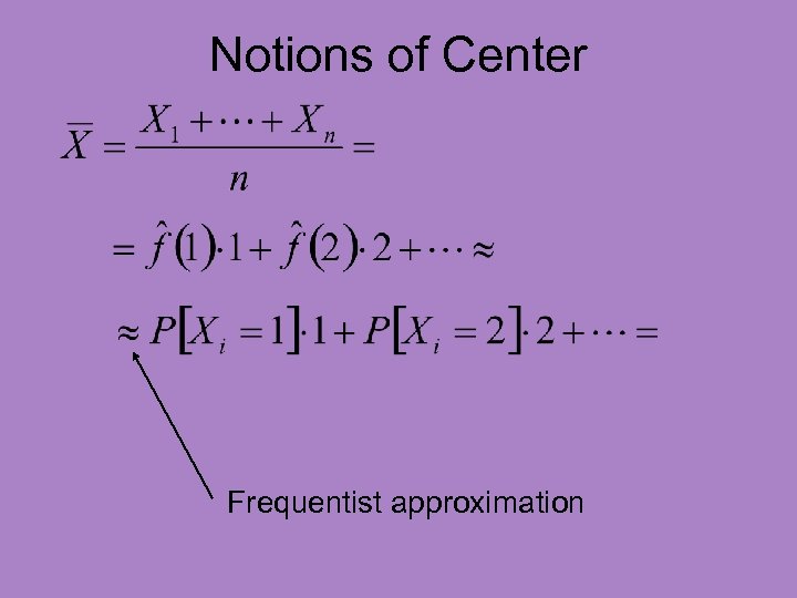
Notions of Center Frequentist approximation

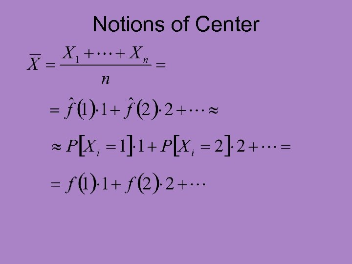
Notions of Center

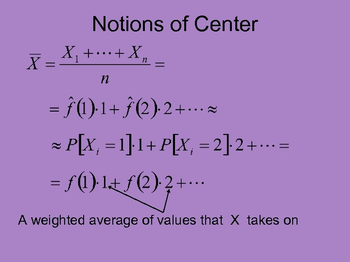
Notions of Center A weighted average of values that X takes on

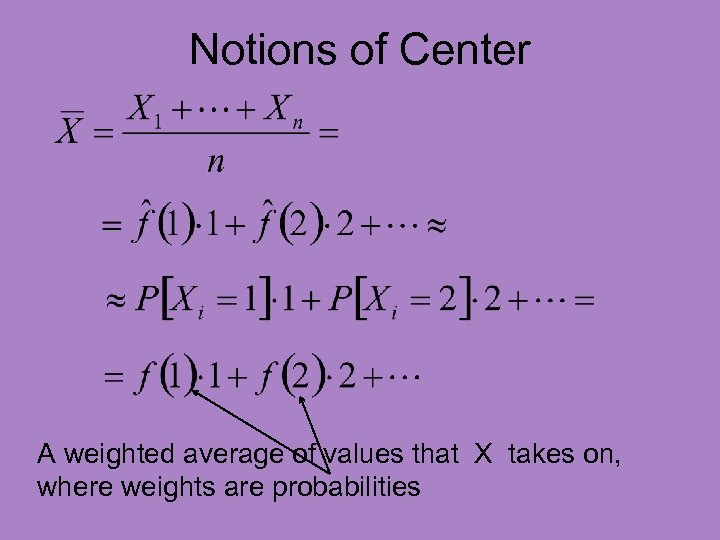
Notions of Center A weighted average of values that X takes on, where weights are probabilities

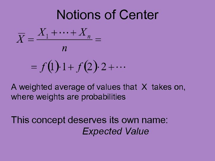
Notions of Center A weighted average of values that X takes on, where weights are probabilities This concept deserves its own name: Expected Value

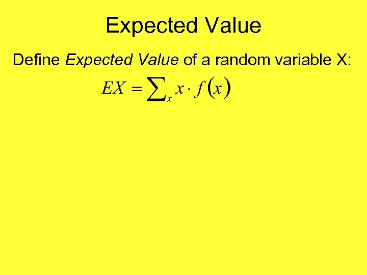
Expected Value Define Expected Value of a random variable X:

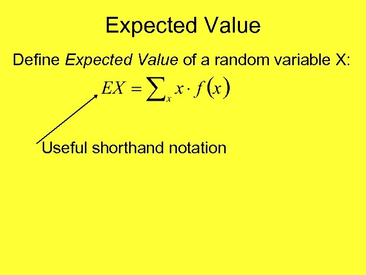
Expected Value Define Expected Value of a random variable X: Useful shorthand notation

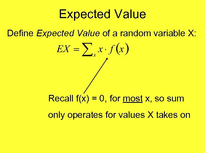
Expected Value Define Expected Value of a random variable X: Recall f(x) = 0, for most x, so sum only operates for values X takes on

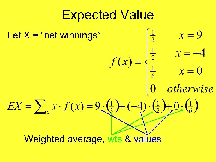
Expected Value E. g. Roll a die, bet (as before):

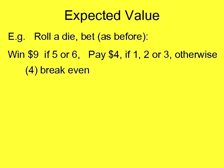
Expected Value E. g. Roll a die, bet (as before): Win $9 if 5 or 6, Pay $4, if 1, 2 or 3, otherwise (4) break even

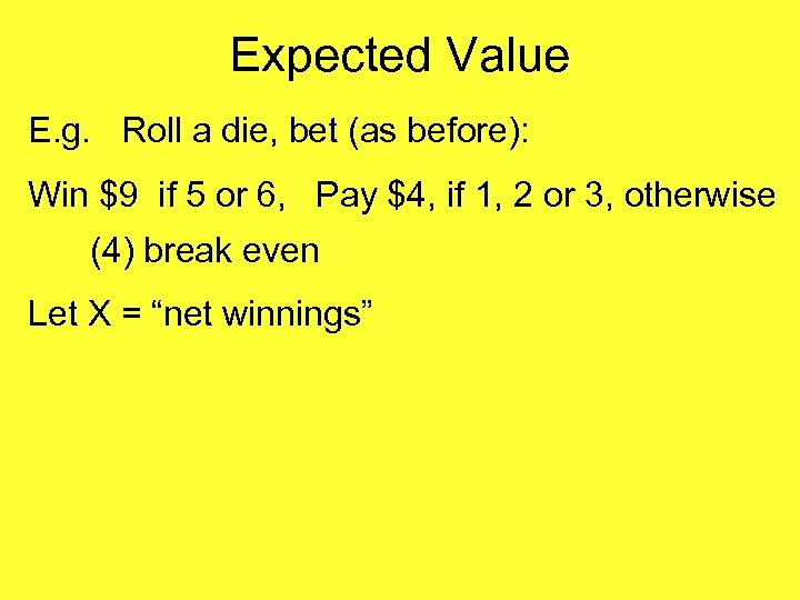
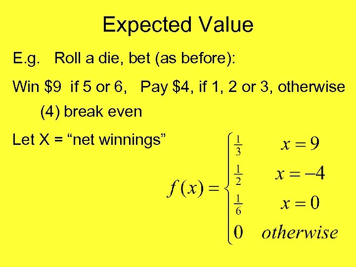
Expected Value E. g. Roll a die, bet (as before): Win $9 if 5 or 6, Pay $4, if 1, 2 or 3, otherwise (4) break even Let X = “net winnings”

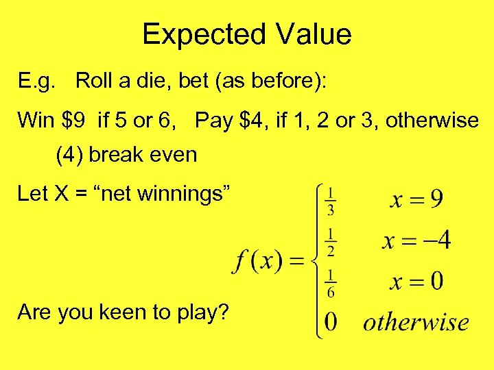
Expected Value E. g. Roll a die, bet (as before): Win $9 if 5 or 6, Pay $4, if 1, 2 or 3, otherwise (4) break even Let X = “net winnings” Are you keen to play?

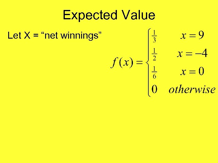
Expected Value Let X = “net winnings”

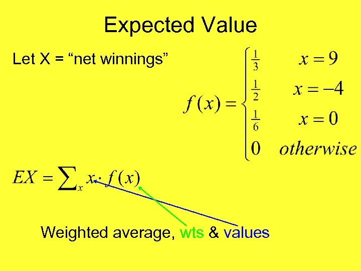
Expected Value Let X = “net winnings” Weighted average, wts & values

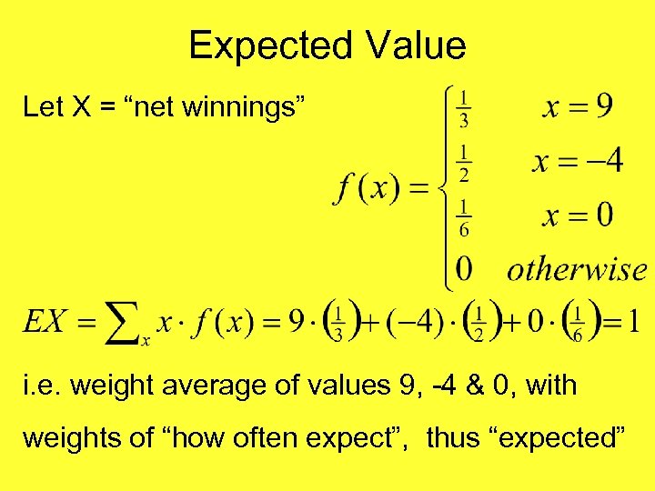
Expected Value Let X = “net winnings” i. e. weight average of values 9, -4 & 0, with weights of “how often expect”, thus “expected”

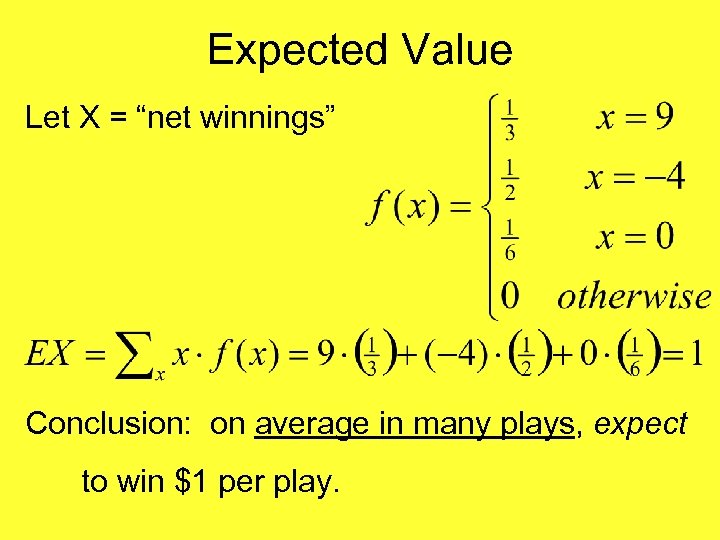
Expected Value Let X = “net winnings” Conclusion: on average in many plays, expect to win $1 per play.

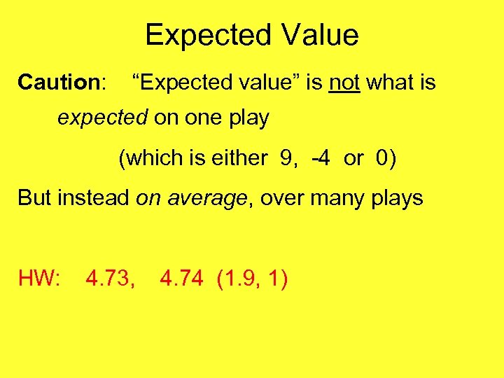
Expected Value Caution: “Expected value” is not what is expected on one play (which is either 9, -4 or 0) But instead on average, over many plays HW: 4. 73, 4. 74 (1. 9, 1)

Expected Value Real life applications of expected value: • Decision Theory – Operations Research – Rational basis for making business decisions – In presence of uncertainty – Common Goal: maximize expected profits – Gives good average results over long run

Expected Value Real life applications of expected value: • Decision Theory • Casino Gambling – Casino offers games with + expected value (+ from their perspective) – Their goal: good overall average performance – Expected Value is a useful tool for this

Expected Value Real life applications of expected value: • Decision Theory • Casino Gambling • Insurance – Companies make profit – By writing policies with + expected value – Their goal is long run average performance

Expected Value Real life applications of expected value: • Decision Theory • Casino Gambling • Insurance • State Lotteries – State’s view: games with + expected value – Raise money for state in long run overall

Flip Side of Expected Value Decisions made against expected value:

Flip Side of Expected Value Decisions made against expected value: • Casino Gambling – Why do people play?

Flip Side of Expected Value Decisions made against expected value: • Casino Gambling – Why do people play? – Odds are against them – For sure will lose “over long run”

Flip Side of Expected Value Decisions made against expected value: • Casino Gambling – Why do people play? – Odds are against them – For sure will lose “over long run” – But love of short run successes, can make eventual long term loss worthwhile – Are buying entertainment

Flip Side of Expected Value Decisions made against expected value: • Casino Gambling • Insurance – Why should you buy it?

Flip Side of Expected Value Decisions made against expected value: • Casino Gambling • Insurance – Why should you buy it? – You lose in expected value sense

Flip Side of Expected Value Decisions made against expected value: • Casino Gambling • Insurance – Why should you buy it? – You lose in expected value sense – But E not applicable since you only play once – Avoids chance of catastrophic loss – Allows low cost sharing of risk

Flip Side of Expected Value Decisions made against expected value: • Casino Gambling • Insurance • State Lotteries – Why do people play?

Flip Side of Expected Value Decisions made against expected value: • Casino Gambling • Insurance • State Lotteries – Why do people play? – Clear loss in expected value

Flip Side of Expected Value Decisions made against expected value: • Casino Gambling • Insurance • State Lotteries – Why do people play? – Clear loss in expected value – But only play once (hopefull), so not applicable – Worth feeling of hope from buying ticket?

Flip Side of Expected Value Interesting issues about State Lotteries: A very different type of tax Big Plus: • Only totally voluntary tax Big Minus: • Tax paid mostly by poor

Flip Side of Expected Value Decisions made against expected value: Key Lesson: Expected Value tells what happens on average over long run, not in one play

Flip Side of Expected Value Decisions made against expected value: Key Lesson: Expected Value tells what happens on average over long run, not in one play Conclude Expected Value not good for everything, but very good for many things

Another Inverse View of Expected Value Suppose you have $5000, and need $10, 000

Another Inverse View of Expected Value Suppose you have $5000, and need $10, 000 e. g. you owe mafia $5000 (gambling debt? ), clean out safe at work for $5000.

Another Inverse View of Expected Value Suppose you have $5000, and need $10, 000 e. g. you owe mafia $5000 (gambling debt? ), clean out safe at work for $5000. If give to mafia, you go to jail

Another Inverse View of Expected Value Suppose you have $5000, and need $10, 000 e. g. you owe mafia $5000 (gambling debt? ), clean out safe at work for $5000. If give to mafia, you go to jail, so decide to raise another $5000 by gambling.

Another Inverse View of Expected Value Suppose you have $5000, and need $10, 000 and can make even bets, with P[win] = 0. 48

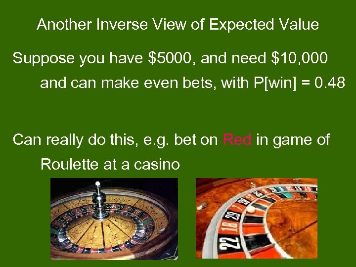
Another Inverse View of Expected Value Suppose you have $5000, and need $10, 000 and can make even bets, with P[win] = 0. 48 Can really do this, e. g. bet on Red in game of Roulette at a casino

Another Inverse View of Expected Value Suppose you have $5000, and need $10, 000 and can make even bets, with P[win] = 0. 48 Important question: Make one large bet? Or many small bets? Something in between?

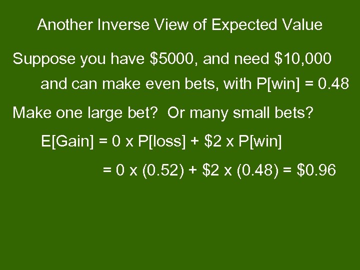
Another Inverse View of Expected Value Suppose you have $5000, and need $10, 000 and can make even bets, with P[win] = 0. 48 Make one large bet? Or many small bets? E[Gain] = 0 x P[loss] + $2 x P[win] = 0 x (0. 52) + $2 x (0. 48) = $0. 96

Another Inverse View of Expected Value Suppose you have $5000, and need $10, 000 and can make even bets, with P[win] = 0. 48 Make one large bet? Or many small bets? E[Gain] = $0. 96 Interpretation: “expect” to lose $0. 04 every time you play

Another Inverse View of Expected Value Suppose you have $5000, and need $10, 000 and can make even bets, with P[win] = 0. 48 Make one large bet? Or many small bets? E[Gain] = $0. 96 Interpretation: “expect” to lose $0. 04 every time you play Why games are so profitable for casinos

Another Inverse View of Expected Value Suppose you have $5000, and need $10, 000 and can make even bets, with P[win] = 0. 48 Make one large bet? Or many small bets? E[Gain] = $0. 96 Interpretation: “expect” to lose $0. 04 every time you play Many plays Expected Value dictates result

Another Inverse View of Expected Value Suppose you have $5000, and need $10, 000 and can make even bets, with P[win] = 0. 48 Make one large bet? Or many small bets? E[Gain] = $0. 96 Interpretation: “expect” to lose $0. 04 every time you play So best to make just one large bet!

Another Inverse View of Expected Value Interpretation: “expect” to lose $0. 04 every time you play So best to make just one large bet!

Another Inverse View of Expected Value Interpretation: “expect” to lose $0. 04 every time you play So best to make just one large bet! After many plays, will surely lose! (lesson of expected value)

Another Inverse View of Expected Value Another View: Strategy one $5000 bet P[win $1, 0000] 0. 48 ≈ ½

Another Inverse View of Expected Value Another View: Strategy P[win $1, 0000] one $5000 bet 0. 48 ≈ ½ two $2500 bets ≈ (0. 48)2 ≈ ¼

Another Inverse View of Expected Value Another View: Strategy P[win $1, 0000] one $5000 bet 0. 48 ≈ ½ two $2500 bets ≈ (0. 48)2 ≈ ¼ four $1250 bets ≈ 1/16

Another Inverse View of Expected Value Another View: Strategy P[win $1, 0000] one $5000 bet 0. 48 ≈ ½ two $2500 bets ≈ (0. 48)2 ≈ ¼ four $1250 bets many bets ≈ 1/16 no chance

Another Inverse View of Expected Value Interpretation: “expect” to lose $0. 04 every time you play So best to make just one large bet! Casino Folklore: Sometimes people really make such bets

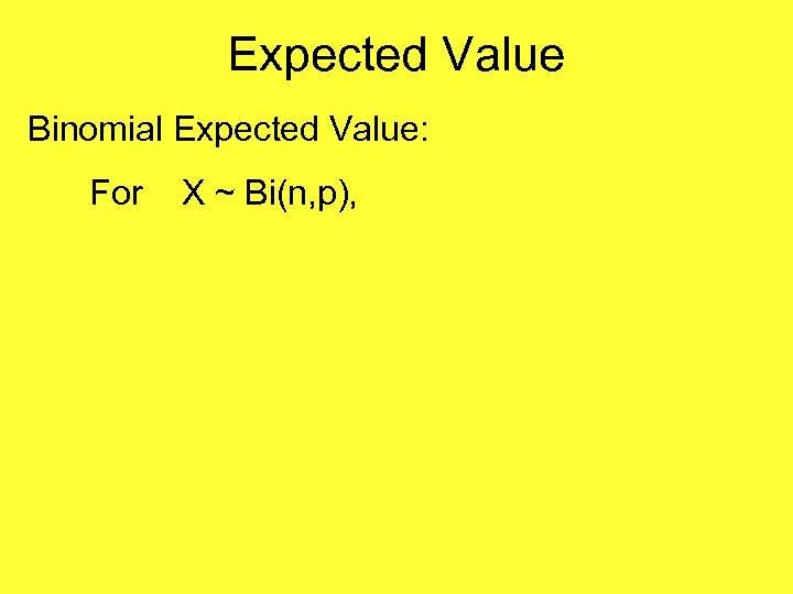
Expected Value Binomial Expected Value: For X ~ Bi(n, p),

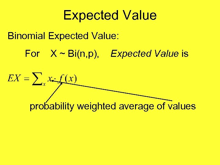
Expected Value Binomial Expected Value: For X ~ Bi(n, p), Expected Value is probability weighted average of values

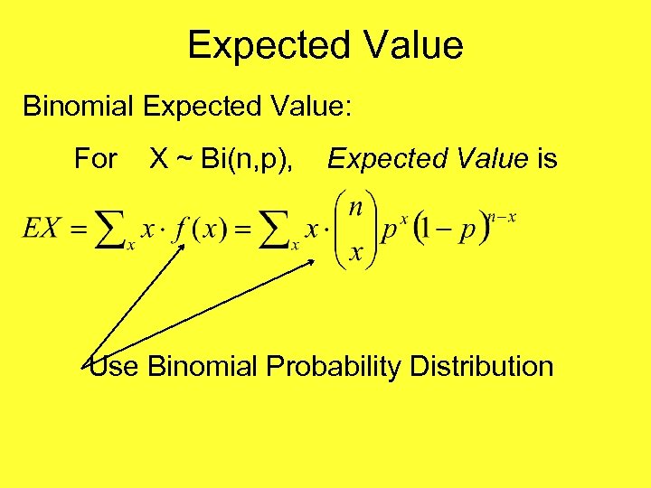
Expected Value Binomial Expected Value: For X ~ Bi(n, p), Expected Value is Use Binomial Probability Distribution

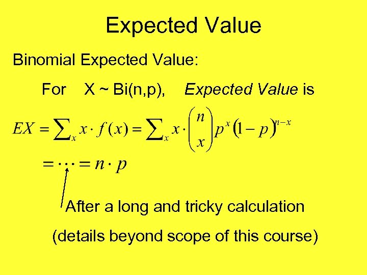
Expected Value Binomial Expected Value: For X ~ Bi(n, p), Expected Value is After a long and tricky calculation (details beyond scope of this course)

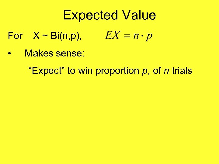
Expected Value For • X ~ Bi(n, p), Makes sense: “Expect” to win proportion p, of n trials

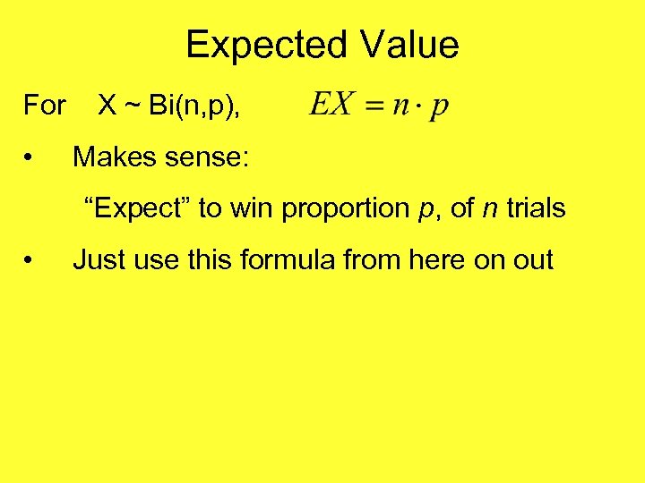
Expected Value For • X ~ Bi(n, p), Makes sense: “Expect” to win proportion p, of n trials • Just use this formula from here on out

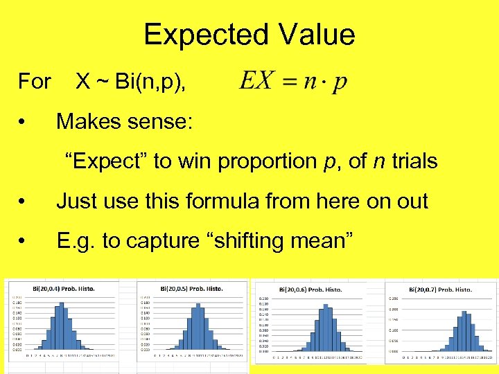
Expected Value For • X ~ Bi(n, p), Makes sense: “Expect” to win proportion p, of n trials • Just use this formula from here on out • E. g. to capture “shifting mean”

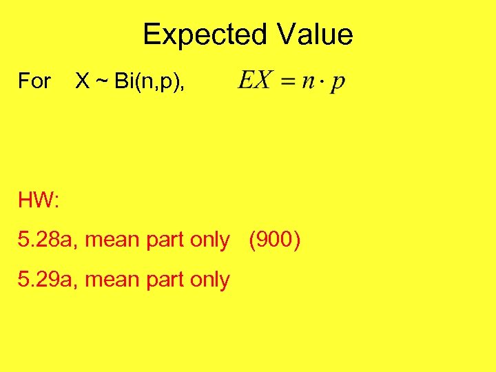
Expected Value For X ~ Bi(n, p), HW: 5. 28 a, mean part only (900) 5. 29 a, mean part only

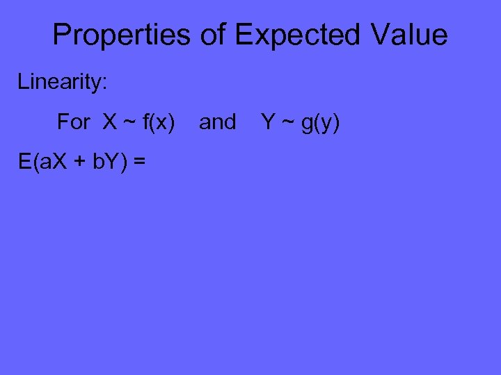
Properties of Expected Value Linearity: For X ~ f(x) E(a. X + b. Y) = and Y ~ g(y)

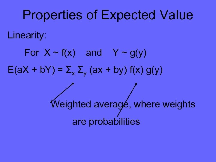
Properties of Expected Value Linearity: For X ~ f(x) and Y ~ g(y) E(a. X + b. Y) = Σx Σy (ax + by) f(x) g(y) Weighted average, where weights are probabilities

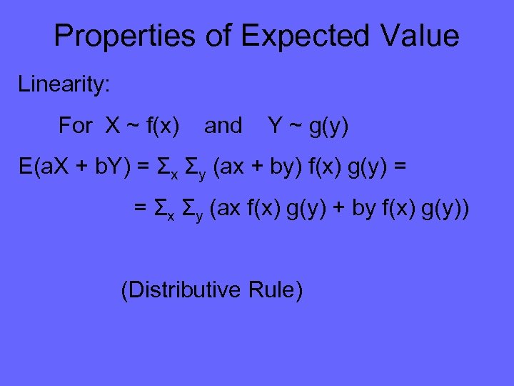
Properties of Expected Value Linearity: For X ~ f(x) and Y ~ g(y) E(a. X + b. Y) = Σx Σy (ax + by) f(x) g(y) = = Σx Σy (ax f(x) g(y) + by f(x) g(y)) (Distributive Rule)

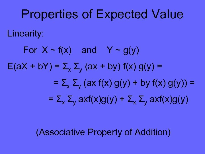
Properties of Expected Value Linearity: For X ~ f(x) and Y ~ g(y) E(a. X + b. Y) = Σx Σy (ax + by) f(x) g(y) = = Σx Σy (ax f(x) g(y) + by f(x) g(y)) = = Σx Σy axf(x)g(y) + Σx Σy axf(x)g(y) (Associative Property of Addition)

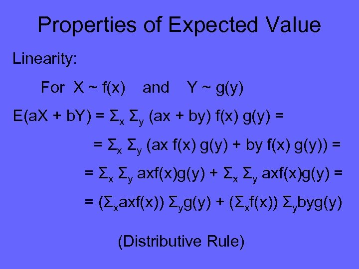
Properties of Expected Value Linearity: For X ~ f(x) and Y ~ g(y) E(a. X + b. Y) = Σx Σy (ax + by) f(x) g(y) = = Σx Σy (ax f(x) g(y) + by f(x) g(y)) = = Σx Σy axf(x)g(y) + Σx Σy axf(x)g(y) = = (Σxaxf(x)) Σyg(y) + (Σxf(x)) Σybyg(y) (Distributive Rule)

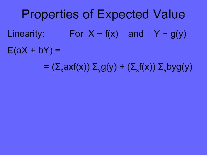
Properties of Expected Value Linearity: For X ~ f(x) and Y ~ g(y) E(a. X + b. Y) = = (Σxaxf(x)) Σyg(y) + (Σxf(x)) Σybyg(y)

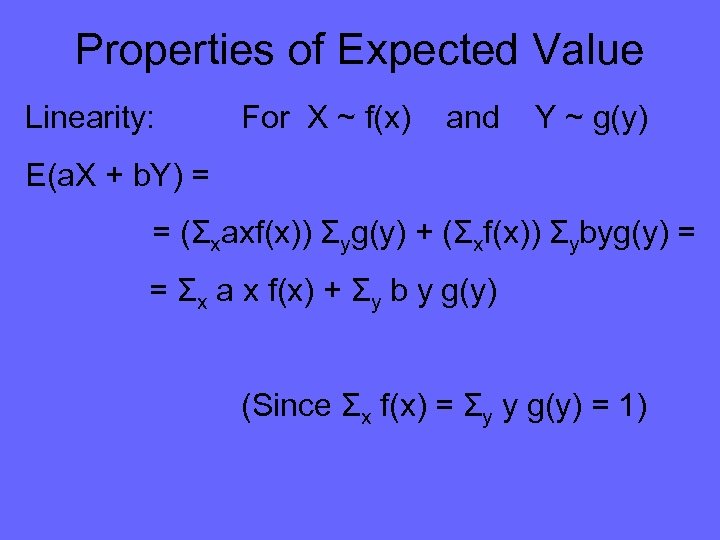
Properties of Expected Value Linearity: For X ~ f(x) and Y ~ g(y) E(a. X + b. Y) = = (Σxaxf(x)) Σyg(y) + (Σxf(x)) Σybyg(y) = = Σx a x f(x) + Σy b y g(y) (Since Σx f(x) = Σy y g(y) = 1)

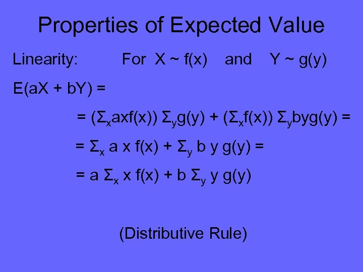
Properties of Expected Value Linearity: For X ~ f(x) and Y ~ g(y) E(a. X + b. Y) = = (Σxaxf(x)) Σyg(y) + (Σxf(x)) Σybyg(y) = = Σx a x f(x) + Σy b y g(y) = = a Σx x f(x) + b Σy y g(y) (Distributive Rule)

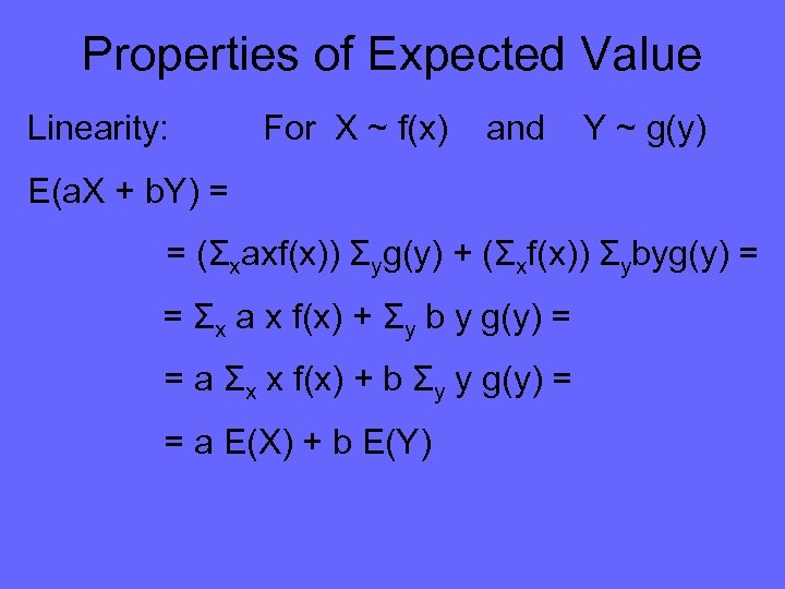
Properties of Expected Value Linearity: For X ~ f(x) and Y ~ g(y) E(a. X + b. Y) = = (Σxaxf(x)) Σyg(y) + (Σxf(x)) Σybyg(y) = = Σx a x f(x) + Σy b y g(y) = = a Σx x f(x) + b Σy y g(y) = = a E(X) + b E(Y)

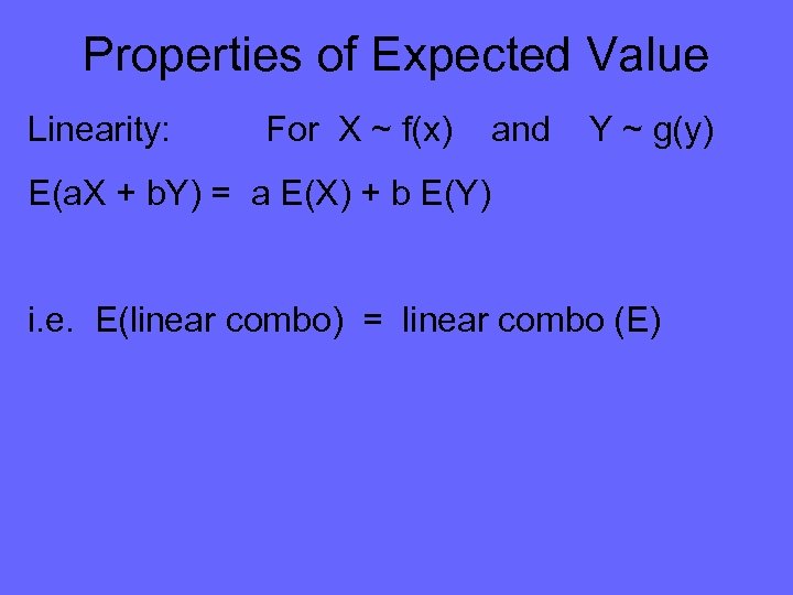
Properties of Expected Value Linearity: For X ~ f(x) and Y ~ g(y) E(a. X + b. Y) = a E(X) + b E(Y) i. e. E(linear combo) = linear combo (E)

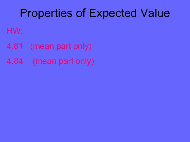
Properties of Expected Value HW: 4. 81 (mean part only) 4. 84 (mean part only)

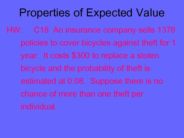
Properties of Expected Value HW: C 18 An insurance company sells 1378 policies to cover bicycles against theft for 1 year. It costs $300 to replace a stolen bicycle and the probability of theft is estimated at 0. 08. Suppose there is no chance of more than one theft per individual.

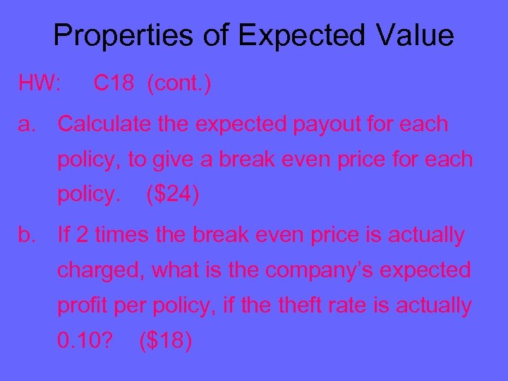
Properties of Expected Value HW: C 18 (cont. ) a. Calculate the expected payout for each policy, to give a break even price for each policy. ($24) b. If 2 times the break even price is actually charged, what is the company’s expected profit per policy, if theft rate is actually 0. 10? ($18)

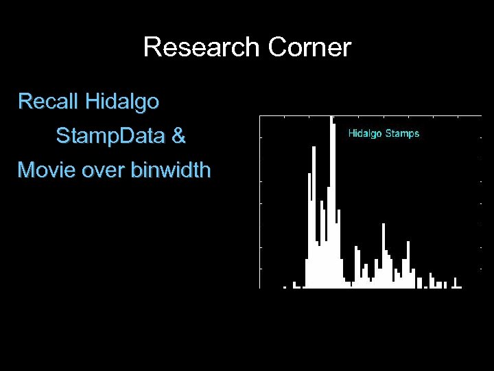
Research Corner Recall Hidalgo Stamp. Data & Movie over binwidth

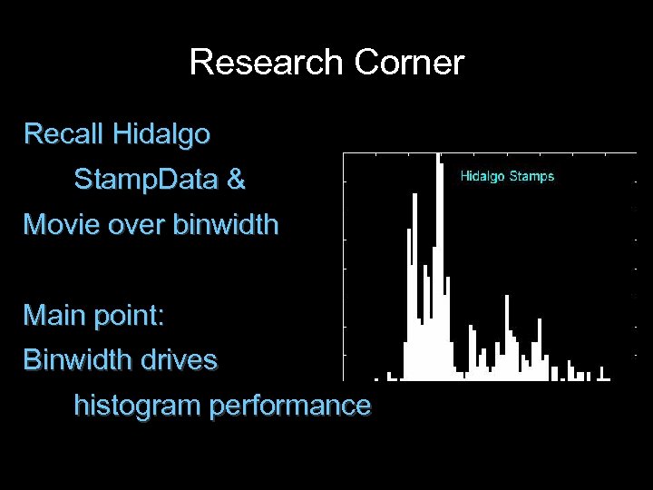
Research Corner Recall Hidalgo Stamp. Data & Movie over binwidth Main point: Binwidth drives histogram performance

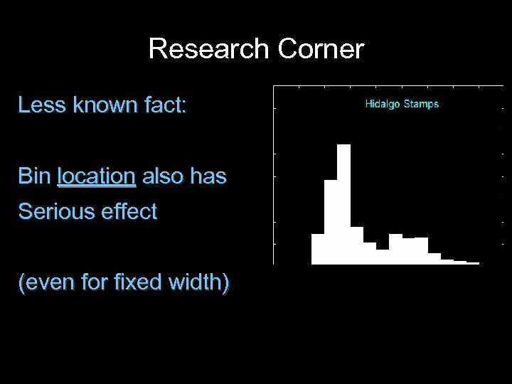
Research Corner Less known fact: Bin location also has Serious effect (even for fixed width)

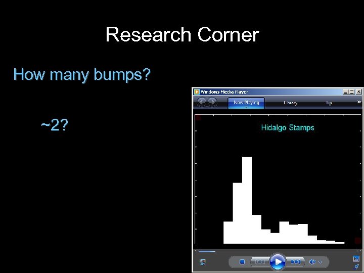
Research Corner How many bumps? ~2?

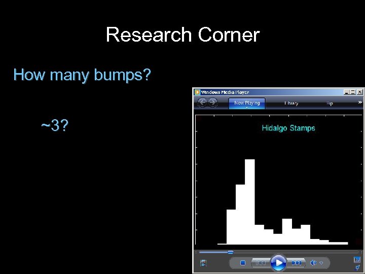
Research Corner How many bumps? ~3?

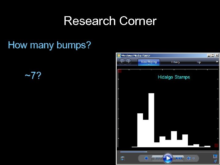
Research Corner How many bumps? ~7?

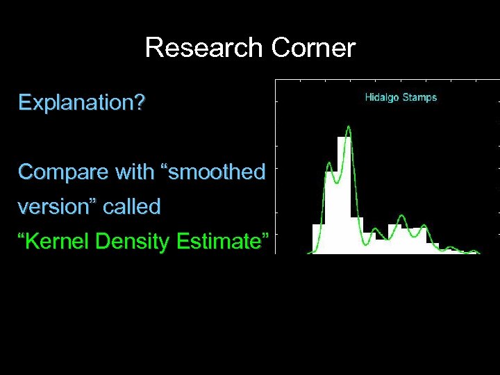
Research Corner Explanation? Compare with “smoothed version” called “Kernel Density Estimate”

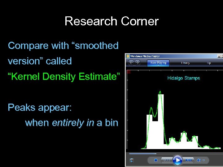
Research Corner Compare with “smoothed version” called “Kernel Density Estimate” Peaks appear: when entirely in a bin

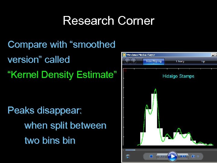
Research Corner Compare with “smoothed version” called “Kernel Density Estimate” Peaks disappear: when split between two bins bin

Research Corner Question: If understand problem with histogram, using Kernel Density Estimate Then why not use KDE for data analysis? Will explore KDE later.

Notions of Center Caution about mean: Works well for ~symmetric distributions

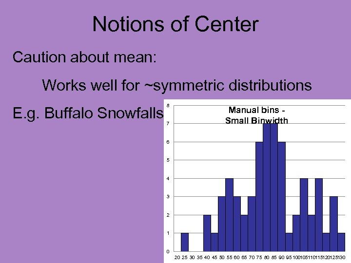
Notions of Center Caution about mean: Works well for ~symmetric distributions E. g. Buffalo Snowfalls 8 7 Manual bins Small Binwidth 6 5 4 3 2 1 0 20 25 30 35 40 45 50 55 60 65 70 75 80 85 90 95 100105110115120125130

Notions of Center Caution about mean: Works well for ~symmetric distributions E. g. Buffalo Snowfalls Analyzed in: http: //www. stat-or. unc. edu/webspace/courses/marron/UNCstor 155 -2009/Class. Notes/Stor 155 Eg 6. xls

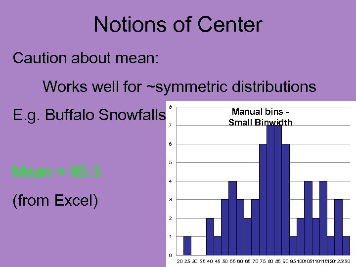
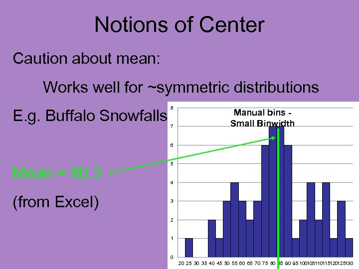
Notions of Center Caution about mean: Works well for ~symmetric distributions E. g. Buffalo Snowfalls 8 7 Manual bins Small Binwidth 6 Mean = 80. 3 (from Excel) 5 4 3 2 1 0 20 25 30 35 40 45 50 55 60 65 70 75 80 85 90 95 100105110115120125130

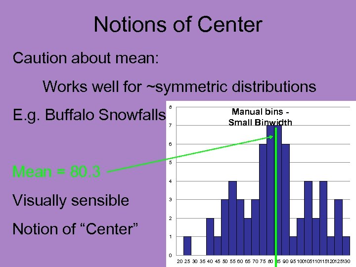
Notions of Center Caution about mean: Works well for ~symmetric distributions E. g. Buffalo Snowfalls 8 7 Manual bins Small Binwidth 6 Mean = 80. 3 Visually sensible Notion of “Center” 5 4 3 2 1 0 20 25 30 35 40 45 50 55 60 65 70 75 80 85 90 95 100105110115120125130

Notions of Center Caution about mean: But poorly for asymmetric distributions

Notions of Center Caution about mean: But poorly for asymmetric distributions E. g. British Suicides Data

Notions of Center Caution about mean: But poorly for asymmetric distributions E. g. British Suicides Data • Time (in days) to suicide attempt • Of Suicide Patients • After Initial Treatment

Notions of Center Caution about mean: But poorly for asymmetric distributions E. g. British Suicides Data Analyzed in: http: //www. stat-or. unc. edu/webspace/courses/marron/UNCstor 155 -2009/Class. Notes/Stor 155 Eg 6. xls

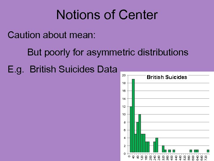
Notions of Center Caution about mean: But poorly for asymmetric distributions 20 British Suicides 18 16 14 12 10 8 6 4 2 0 0 40 80 120 160 200 240 280 320 360 400 440 480 520 560 600 640 680 720 E. g. British Suicides Data

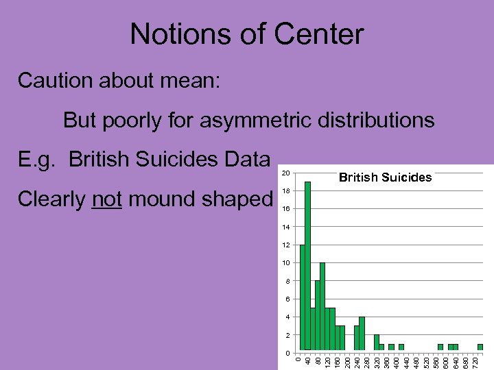
Notions of Center Caution about mean: But poorly for asymmetric distributions Clearly not mound shaped 20 British Suicides 18 16 14 12 10 8 6 4 2 0 0 40 80 120 160 200 240 280 320 360 400 440 480 520 560 600 640 680 720 E. g. British Suicides Data

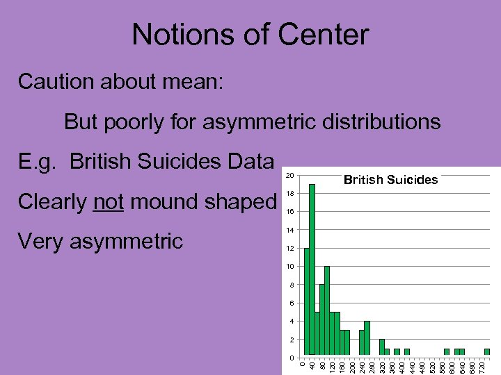
Notions of Center Caution about mean: But poorly for asymmetric distributions E. g. British Suicides Data 20 Clearly not mound shaped 18 Very asymmetric British Suicides 14 16 12 10 8 6 4 0 0 40 80 120 160 200 240 280 320 360 400 440 480 520 560 600 640 680 720 2

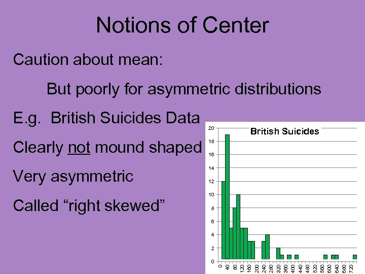
Notions of Center Caution about mean: But poorly for asymmetric distributions E. g. British Suicides Data 20 Clearly not mound shaped 18 Very asymmetric British Suicides 14 12 10 8 6 4 2 0 0 40 80 120 160 200 240 280 320 360 400 440 480 520 560 600 640 680 720 Called “right skewed” 16

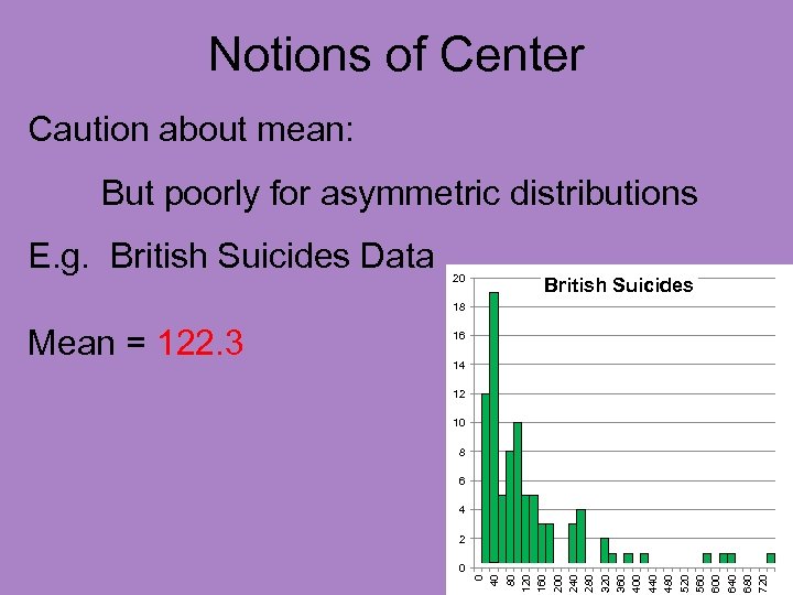
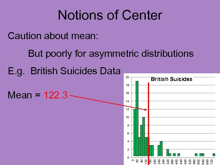
Notions of Center Caution about mean: But poorly for asymmetric distributions E. g. British Suicides Data 20 British Suicides 18 16 14 12 10 8 6 4 2 0 0 40 80 120 160 200 240 280 320 360 400 440 480 520 560 600 640 680 720 Mean = 122. 3

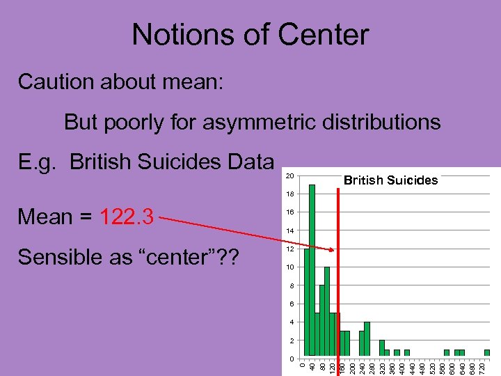
Notions of Center Caution about mean: But poorly for asymmetric distributions E. g. British Suicides Data 20 British Suicides 18 Sensible as “center”? ? 16 14 12 10 8 6 4 2 0 0 40 80 120 160 200 240 280 320 360 400 440 480 520 560 600 640 680 720 Mean = 122. 3

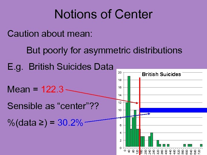
Notions of Center Caution about mean: But poorly for asymmetric distributions E. g. British Suicides Data 20 British Suicides 18 Sensible as “center”? ? %(data ≥) = 30. 2% 16 14 12 10 8 6 4 2 0 0 40 80 120 160 200 240 280 320 360 400 440 480 520 560 600 640 680 720 Mean = 122. 3

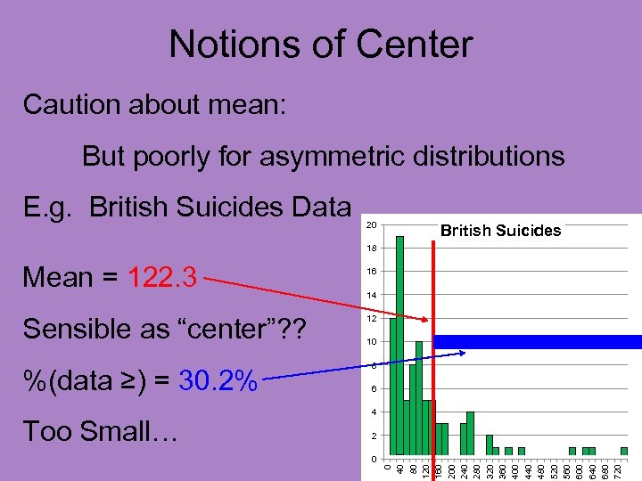
Notions of Center Caution about mean: But poorly for asymmetric distributions E. g. British Suicides Data 20 British Suicides 18 Sensible as “center”? ? %(data ≥) = 30. 2% Too Small… 16 14 12 10 8 6 4 2 0 0 40 80 120 160 200 240 280 320 360 400 440 480 520 560 600 640 680 720 Mean = 122. 3

Notions of Center Perhaps better notion of “center”: • Take center to be point in middle • I. e. have 50% of data smaller • And 50% of data larger This is called the “median”

Notions of Center Median: = Value in middle (of sorted list)

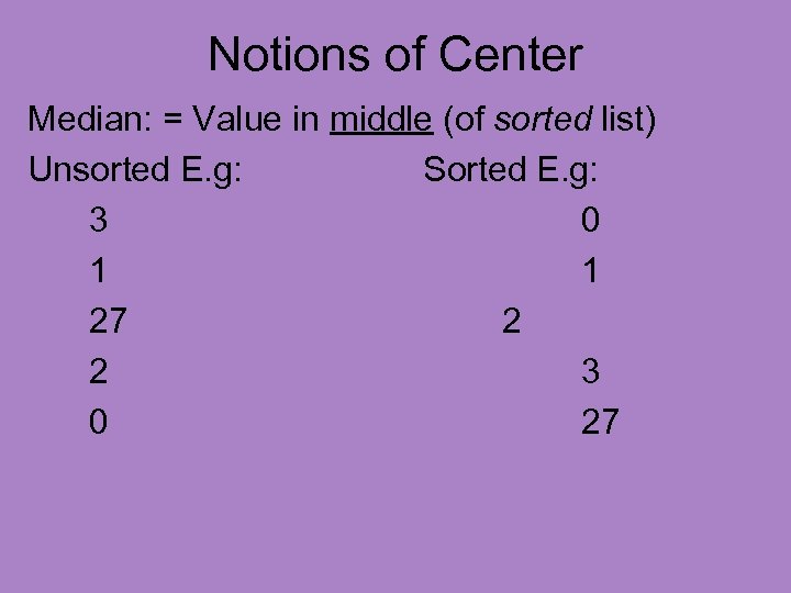
Notions of Center Median: = Value in middle (of sorted list) Unsorted E. g: Sorted E. g: 3 0 1 1 27 2 2 3 0 27

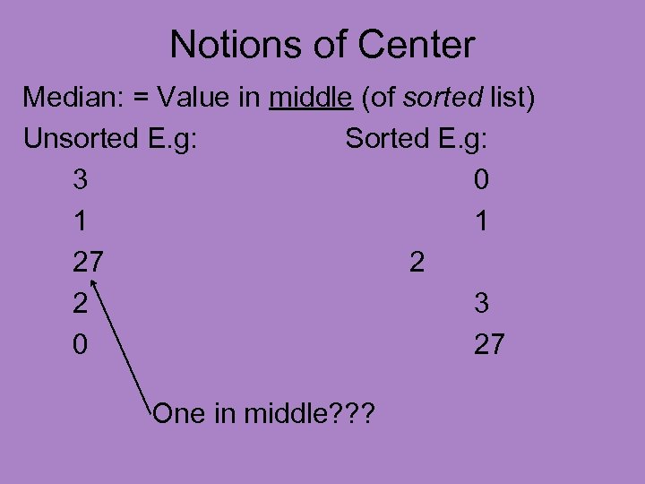
Notions of Center Median: = Value in middle (of sorted list) Unsorted E. g: Sorted E. g: 3 0 1 1 27 2 2 3 0 27 One in middle? ? ?

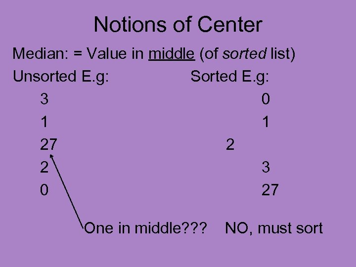
Notions of Center Median: = Value in middle (of sorted list) Unsorted E. g: Sorted E. g: 3 0 1 1 27 2 2 3 0 27 One in middle? ? ? NO, must sort

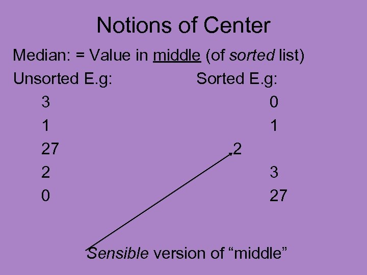
Notions of Center Median: = Value in middle (of sorted list) Unsorted E. g: Sorted E. g: 3 0 1 1 27 2 2 3 0 27 Sensible version of “middle”

Notions of Center What about ties? Sorted E. g: 0 1 2 3

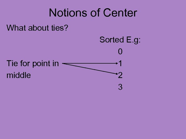
Notions of Center What about ties? Tie for point in middle Sorted E. g: 0 1 2 3

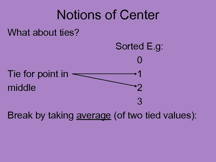
Notions of Center What about ties? Sorted E. g: 0 Tie for point in 1 middle 2 3 Break by taking average (of two tied values):

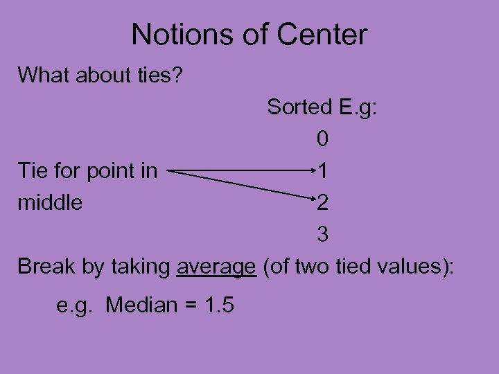
Notions of Center What about ties? Sorted E. g: 0 Tie for point in 1 middle 2 3 Break by taking average (of two tied values): e. g. Median = 1. 5

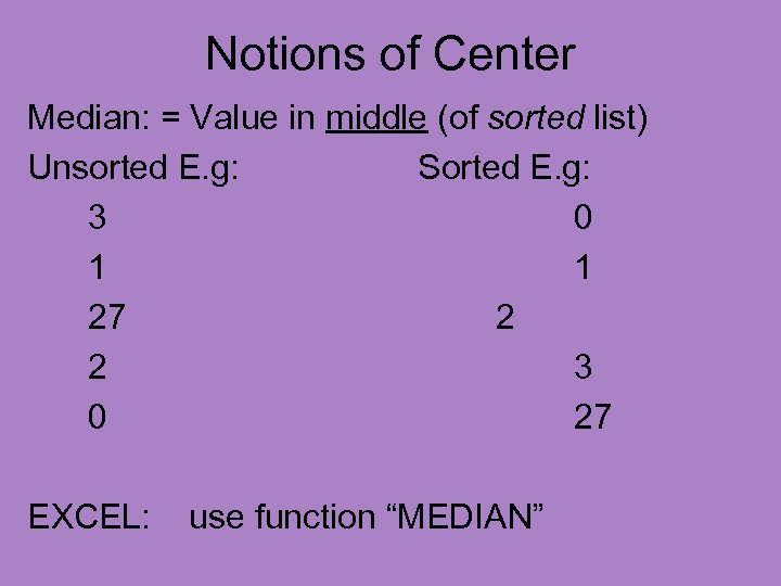
Notions of Center Median: = Value in middle (of sorted list) Unsorted E. g: Sorted E. g: 3 0 1 1 27 2 2 3 0 27 EXCEL: use function “MEDIAN”

Notions of Center EXCEL: use function “MEDIAN” Very similar to other functions E. g. see: http: //www. stat-or. unc. edu/webspace/courses/marron/UNCstor 155 -2009/Class. Notes/Stor 155 Eg 6. xls

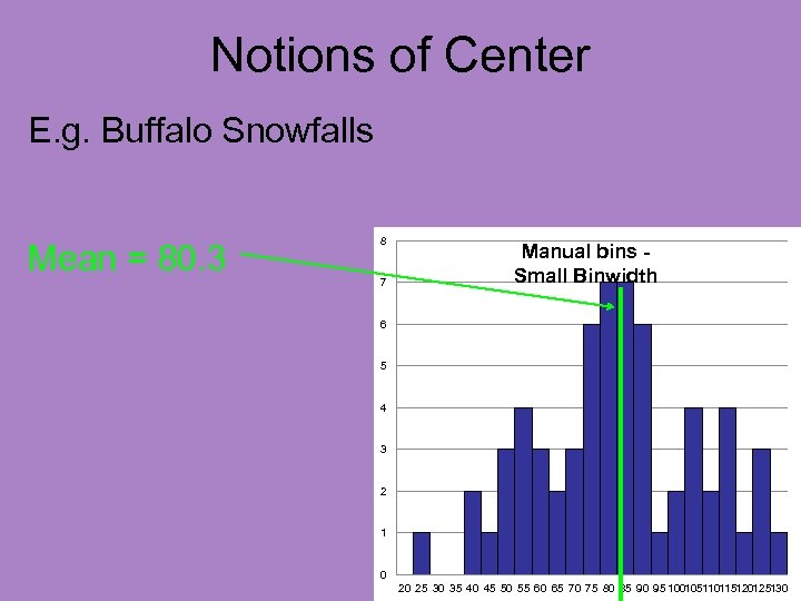
Notions of Center E. g. Buffalo Snowfalls Mean = 80. 3 8 7 Manual bins Small Binwidth 6 5 4 3 2 1 0 20 25 30 35 40 45 50 55 60 65 70 75 80 85 90 95 100105110115120125130

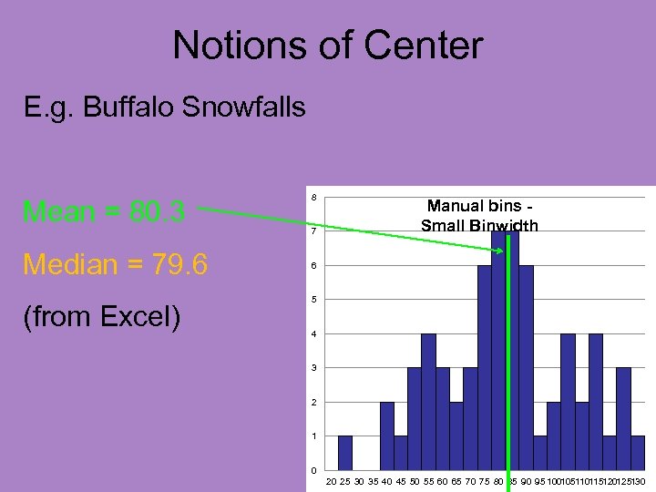
Notions of Center E. g. Buffalo Snowfalls Mean = 80. 3 Median = 79. 6 (from Excel) 8 7 Manual bins Small Binwidth 6 5 4 3 2 1 0 20 25 30 35 40 45 50 55 60 65 70 75 80 85 90 95 100105110115120125130

Notions of Center E. g. Buffalo Snowfalls Mean = 80. 3 Median = 79. 6 Very similar 8 7 Manual bins Small Binwidth 6 5 4 3 2 1 0 20 25 30 35 40 45 50 55 60 65 70 75 80 85 90 95 100105110115120125130

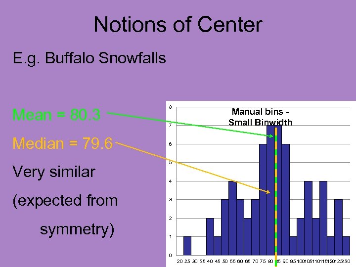
Notions of Center E. g. Buffalo Snowfalls Mean = 80. 3 Median = 79. 6 Very similar (expected from symmetry) 8 7 Manual bins Small Binwidth 6 5 4 3 2 1 0 20 25 30 35 40 45 50 55 60 65 70 75 80 85 90 95 100105110115120125130

Notions of Center E. g. British Suicides Data Mean = 122. 3 Median = 77. 5 20 British Suicides 18 16 14 12 10 8 6 4 2 0 0 40 80 120 160 200 240 280 320 360 400 440 480 520 560 600 640 680 720 Substantially different

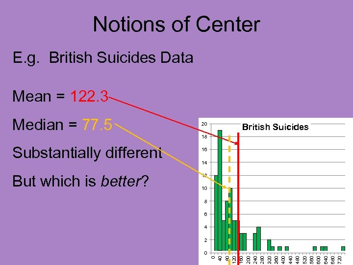
Notions of Center E. g. British Suicides Data Mean = 122. 3 Median = 77. 5 20 British Suicides 18 But which is better? 16 14 12 10 8 6 4 2 0 0 40 80 120 160 200 240 280 320 360 400 440 480 520 560 600 640 680 720 Substantially different

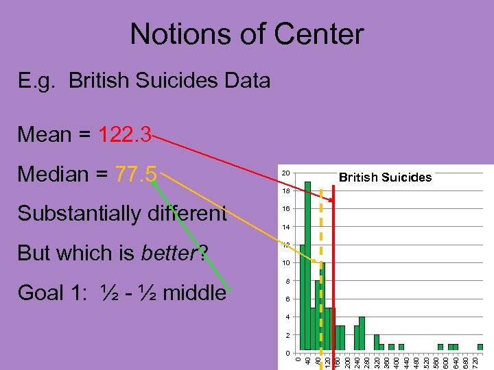
Notions of Center E. g. British Suicides Data Mean = 122. 3 Median = 77. 5 20 British Suicides 18 But which is better? Goal 1: ½ - ½ middle 16 14 12 10 8 6 4 2 0 0 40 80 120 160 200 240 280 320 360 400 440 480 520 560 600 640 680 720 Substantially different

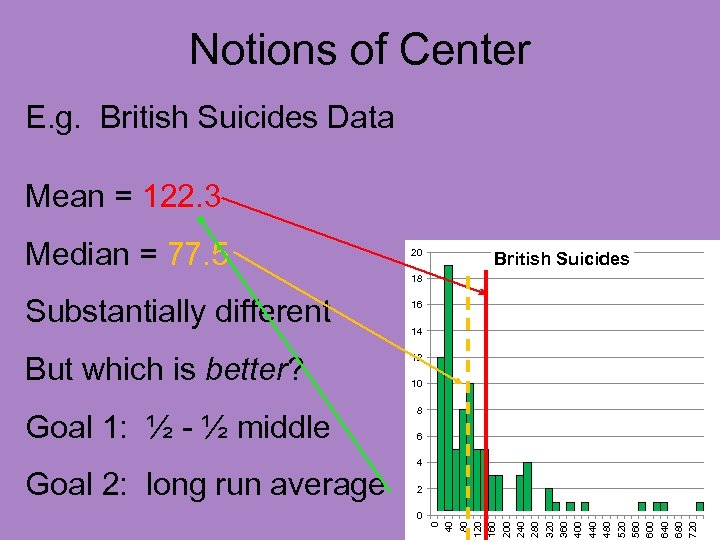
Notions of Center E. g. British Suicides Data Mean = 122. 3 Median = 77. 5 20 British Suicides 18 But which is better? Goal 1: ½ - ½ middle Goal 2: long run average 16 14 12 10 8 6 4 2 0 0 40 80 120 160 200 240 280 320 360 400 440 480 520 560 600 640 680 720 Substantially different