Laboratory of Embedded Control Systems Course Presentation Teacher

Laboratory of Embedded Control Systems Course Presentation Teacher Luigi Palopoli AA. 2011/2012

Aim of the course § The aim of this course it to introduce the student (you : =) ) to model based design of embedded control systems § This will be done with theoretical lectures (few) and lab experiences (many) § The course is a laboratory course. ★ What we expect is that you deliver a complete working project § You will organise yourself in groups of two students ★ Please start searching for your mate and let me know in the next class

The project § The project will be developed in different phases § At the end of each phase, you will produce a different artefact (e. g. , a piece of code or a model), which has to be documented by a report ★ There is a specific date for each delivery ★ Those of you who do not attend the class can deliver the project all at once, but I warmly recommend not to (is possible) § We will do most of the work together in the class, but you may need to work on your own to complete the different phase

What this course is not. . . § It is not a Signals and System course § It is not a Real-Time Operating Systems course § It is not an automatic control or a digital control course. . . . but you will need a little bit of all of this and we will help you. .

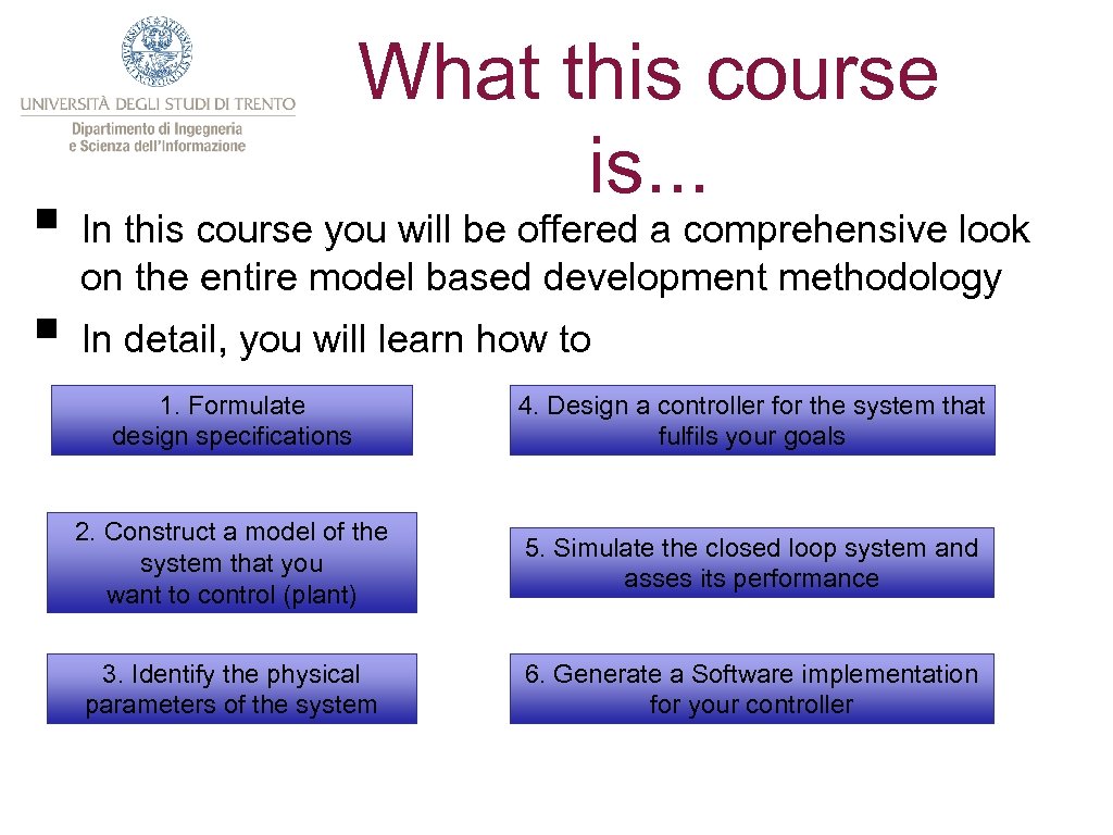
What this course is. . . § In this course you will be offered a comprehensive look on the entire model based development methodology § In detail, you will learn how to 1. Formulate design specifications 4. Design a controller for the system that fulfils your goals 2. Construct a model of the system that you want to control (plant) 5. Simulate the closed loop system and asses its performance 3. Identify the physical parameters of the system 6. Generate a Software implementation for your controller

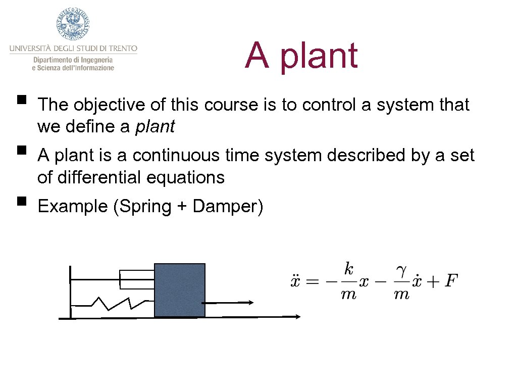
A plant § The objective of this course is to control a system that we define a plant § A plant is a continuous time system described by a set of differential equations § Example (Spring + Damper)

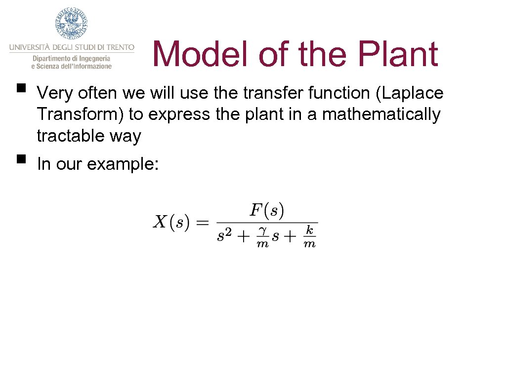
Model of the Plant § Very often we will use the transfer function (Laplace Transform) to express the plant in a mathematically tractable way § In our example:

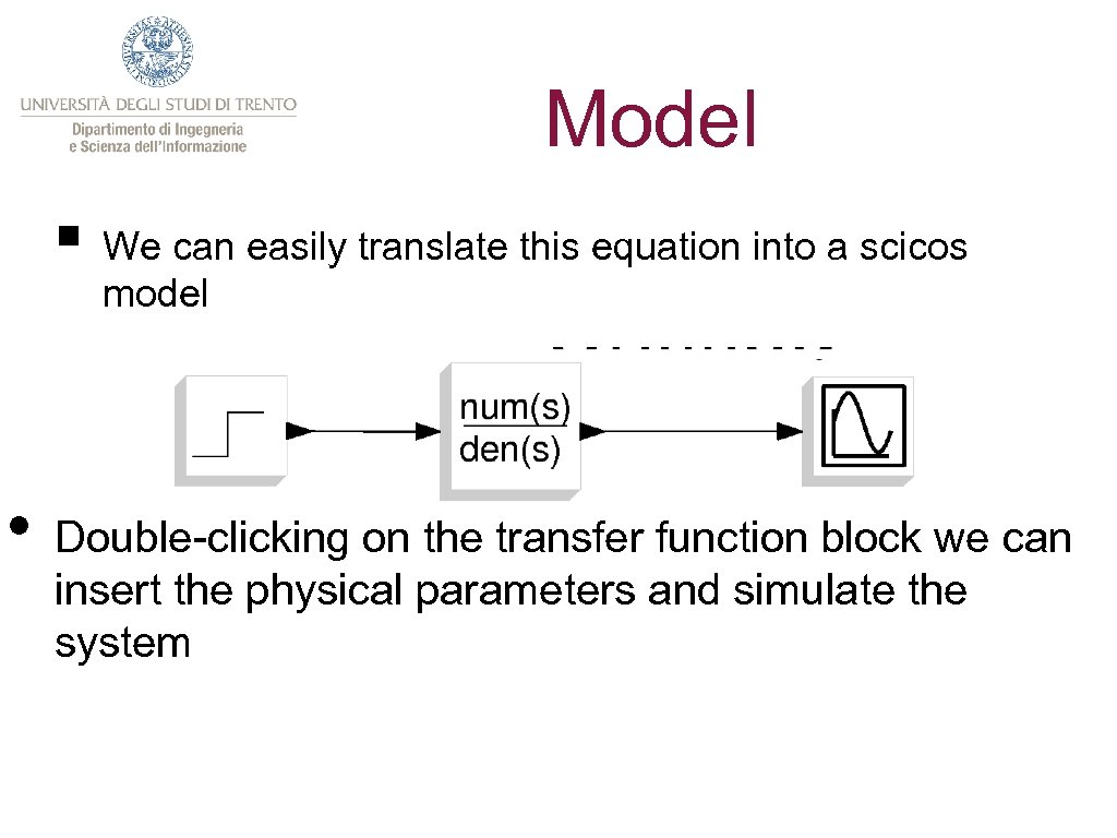
Model § We can easily translate this equation into a scicos model • Double-clicking on the transfer function block we can insert the physical parameters and simulate the system

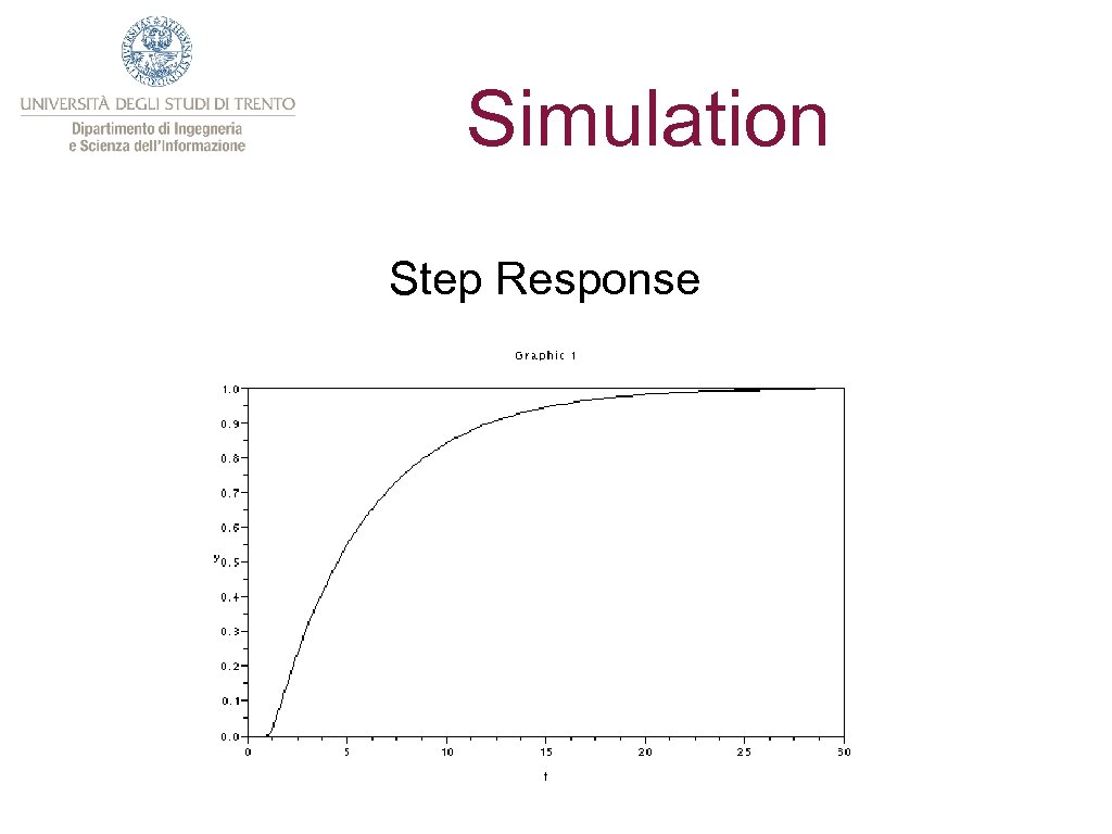
Simulation Step Response

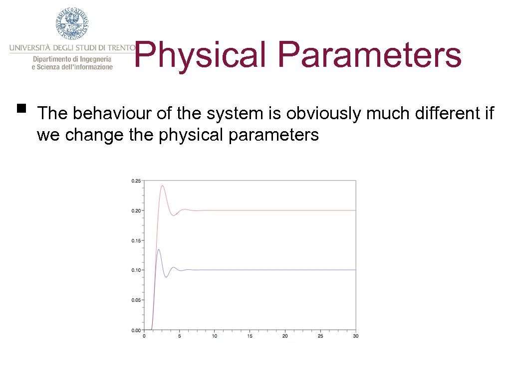
Physical Parameters § The behaviour of the system is obviously much different if we change the physical parameters

§ To make our model. Non-idealities our more realistic, we can refine model inserting blocks that model non-idealities § For instance, actuators are not able to produce any input value ★ an utility car is different from a Formula 1 racing car ★ we can model this by inserting in the model a “saturation” block ★ The system is no longer linear (why? ) but we can consider its behaviour as linear ad long as we do not exceed the bound of the saturation

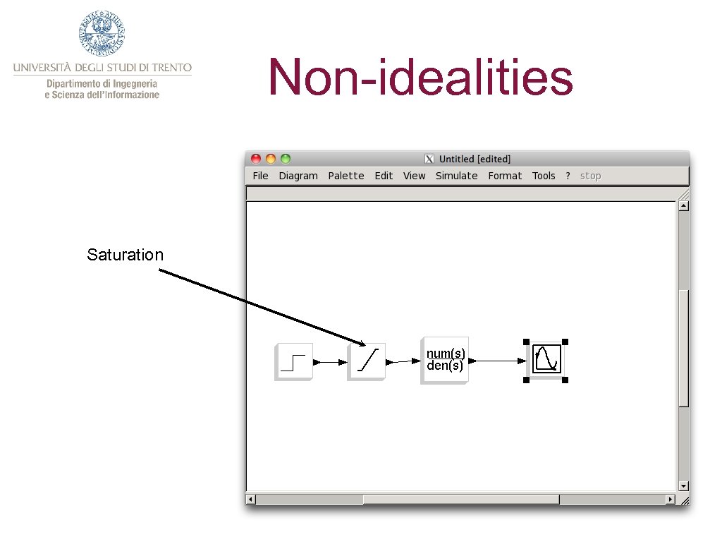
Non-idealities Saturation

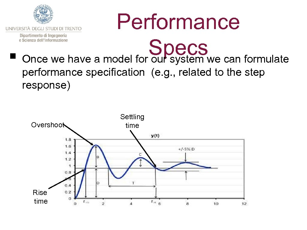
Performance Specswe can formulate § Once we have a model for our system performance specification (e. g. , related to the step response) Overshoot Rise time Settling time

Physical Parameters § Essential to our purpose is to determine the choice of parameters whereby our model best fits the model ★ To do this we can ✴ measure the physical quantities if easy/possible ✴ Carry out the identification procedure § Identification: ★ carry out a large set of experiments and collect data ★ find the set of parameters that minimise the distance between our system and the model

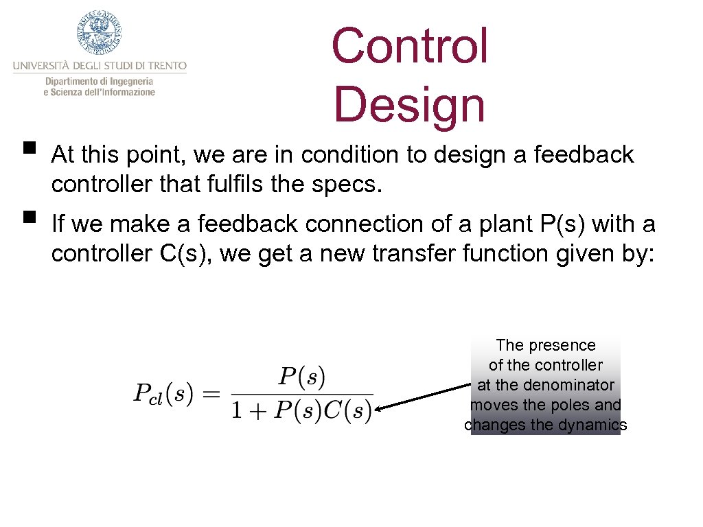
Control Design § At this point, we are in condition to design a feedback controller that fulfils the specs. § If we make a feedback connection of a plant P(s) with a controller C(s), we get a new transfer function given by: The presence of the controller at the denominator moves the poles and changes the dynamics

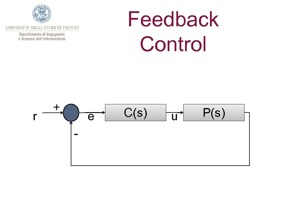
Feedback Control r + e - C(s) u P(s)

Digital Implementation § The controller we have designed in this way is a continuous time system (a differential equation) § If we want to implement it in a digital computer, we need to transform it into a numeric algorithm § Instrumental to this goal is the introduction of a sampling mechanism for the sensors and of a Zero order Hold (Zo. H) for the actuators

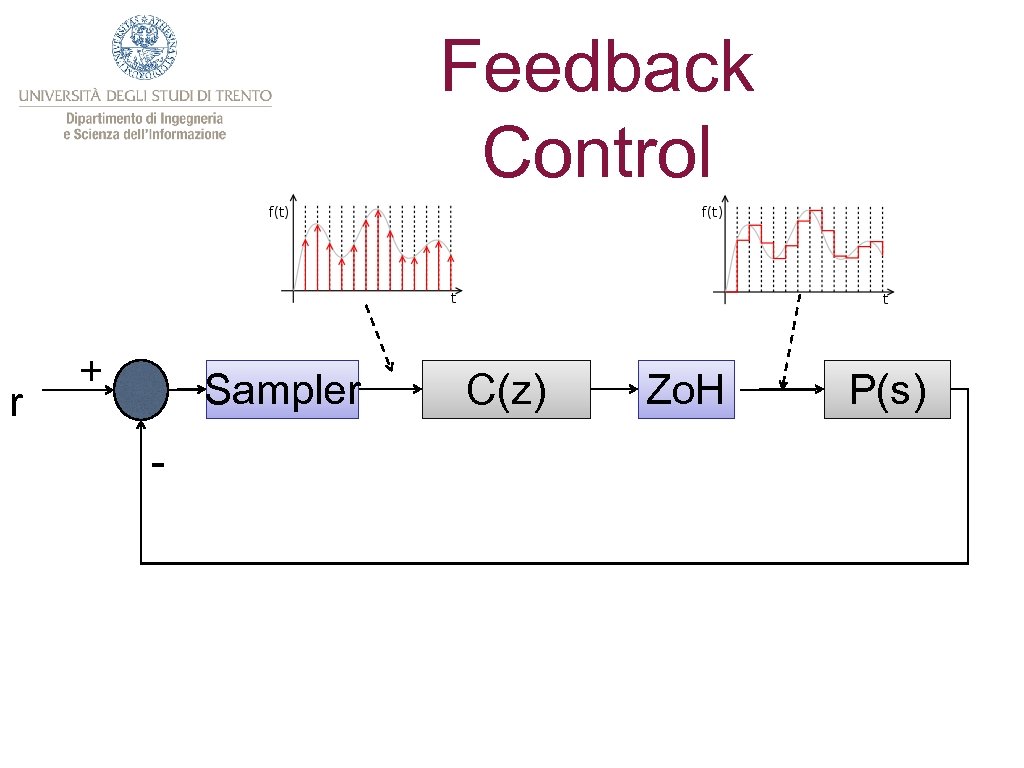
Feedback Control r + Sampler - C(z) Zo. H P(s)

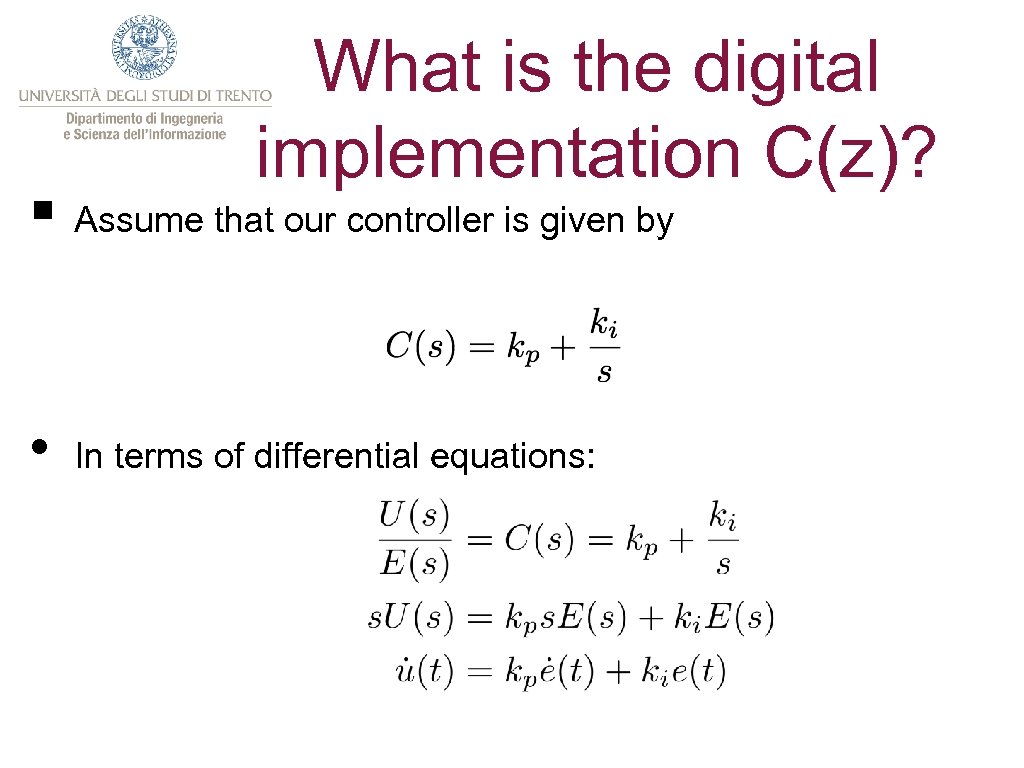
What is the digital implementation C(z)? § Assume that our controller is given by • In terms of differential equations:

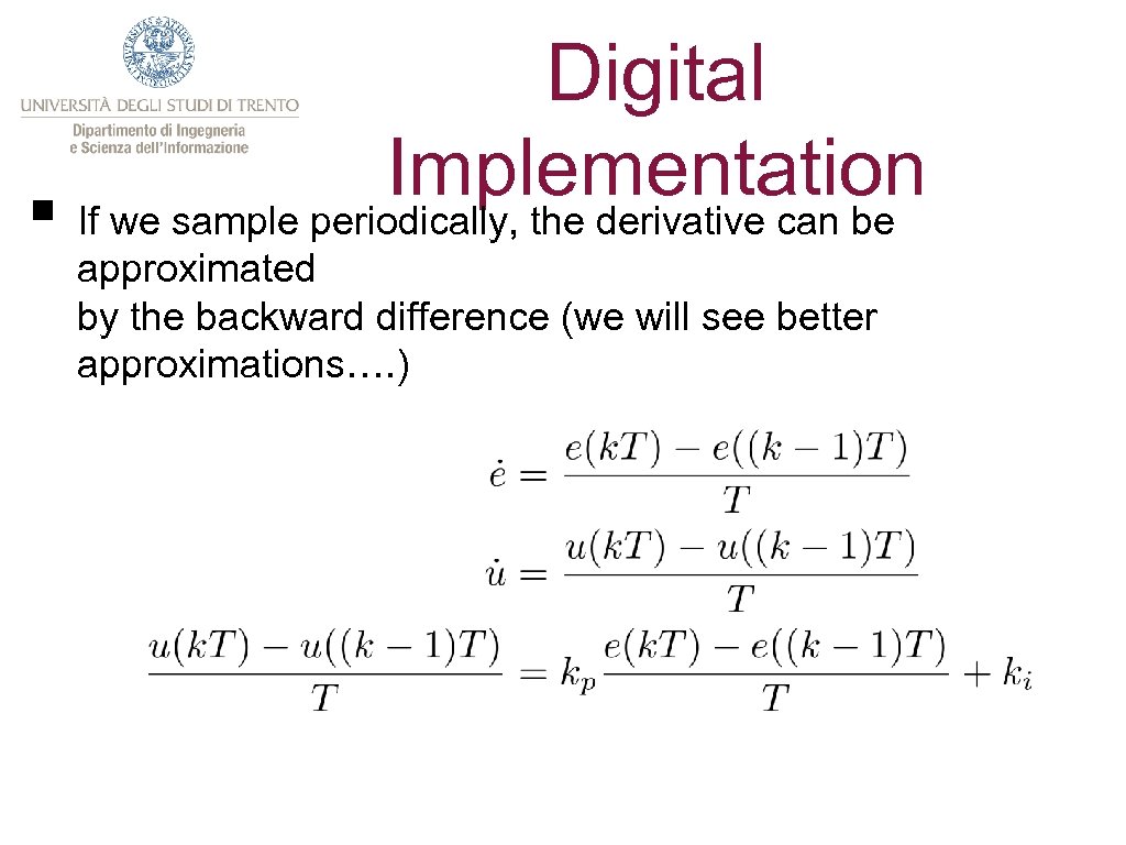
Digital Implementation § If we sample periodically, the derivative can be approximated by the backward difference (we will see better approximations…. )

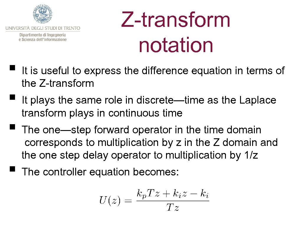
Z-transform notation § It is useful to express the difference equation in terms of the Z-transform § It plays the same role in discrete—time as the Laplace transform plays in continuous time § The one—step forward operator in the time domain corresponds to multiplication by z in the Z domain and the one step delay operator to multiplication by 1/z § The controller equation becomes:

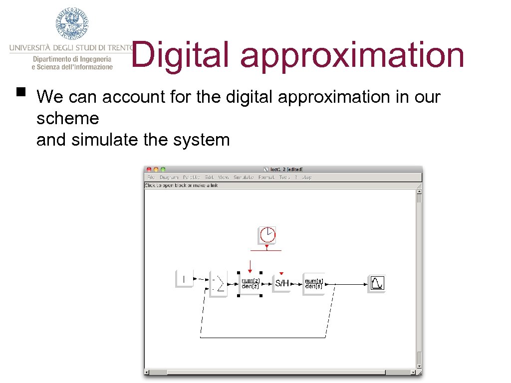
Digital approximation § We can account for the digital approximation in our scheme and simulate the system

…and finally…. § Once we are happy with the simulations, we can write a real—time task (implemented in a RTOS) that translates the algorithm into code double e_1, u_1; void task () { double u, e; e = get_from_sensor(); u = u_1 + kp (e-e_1)+ki*e; output(u); e_1 = e: u_1 = u; }

Schedule § Lecture 1: Introduction ★ Methodology ★ Introduction to Scicoslab § Lecture II: Scicoslab ★ Matrix computation ★ Scripts and functions ★ Plotting data ★ Modelling and simulating a CT system with Scicos

Schedule § Lecture III: Interfacing Scicos. Lab and Lego ★ Setup of the environment (step by step) ★ Example 1: turn on a motor and read the encoder through USB and dump on file ✴ Read the file with Scilab and plot it § Lecture IV: Recap on Laplace transform

Schedule § Lecture V: Modelling a second order system § Lecture VI: Identification of a second order system ★ Scicos-lab examples (identifying a second order system using synthetic data) ★ Filtering

Schedule § Lecture VII: Identification of the Lego’s motors ★ Collection of Data § Lecture VIII: Identification of the Lego’s motors ★ Filtering ★ Identification

Schedule § Lecture IX: Control of SISO system ★ root locus § [DELIVERY] Lecture X: Identification of the Lego’s motors ★ Filtering ★ Identification

Schedule § Lecture XI: Control of SISO system ★ root locus ★ PID § Lecture XII: Example of design using scicoslab ★ Second order systems: from specs to control ★ Assesment by simulation

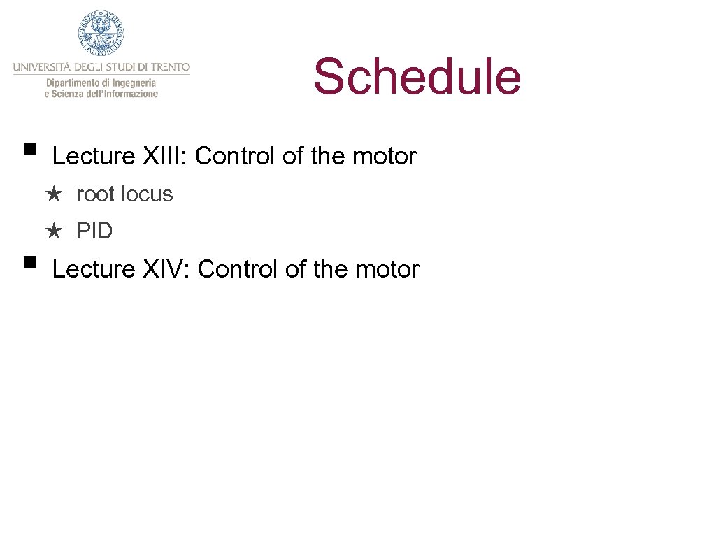
Schedule § Lecture XIII: Control of the motor ★ root locus ★ PID § Lecture XIV: Control of the motor

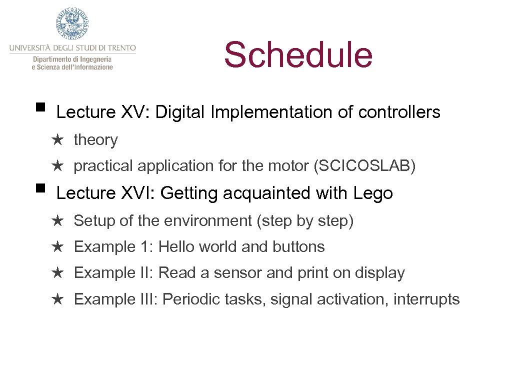
Schedule § Lecture XV: Digital Implementation of controllers ★ theory ★ practical application for the motor (SCICOSLAB) § Lecture XVI: Getting acquainted with Lego ★ Setup of the environment (step by step) ★ Example 1: Hello world and buttons ★ Example II: Read a sensor and print on display ★ Example III: Periodic tasks, signal activation, interrupts

Schedule § Lecture XVII: Modelling and simulation of the larger system § [Delivery] Lecture XVIII: Implementing the digital controller

Schedule § Lecture XIX: Control design based on State Space Methods § Lecture XX: Control design based on State Space Methods

Schedule § Lecture XXI: Design of the control in SCICOLAB § Lecture XXII: Design of the control in SCICOLAB

Schedule § Lecture XXIII: Design of the control in SCICOLAB ★ Digital implementation § Lecture XXIV: Design of the control in SCICOLAB ★ Coding § After 1 Week delivery