Laboratory of Computational Geodynamics Graduate University of Chinese

Laboratory of Computational Geodynamics, Graduate University of Chinese Academy of Sciences Multi-Scale Parallel computing in Laboratory of Computational Geodynamics, Chinese Academy of Sciences Yaolin Shi 1, Mian Liu 2, 1, Huai Zhang 1, David A. Yuen 3 , Hui Wang 1, Shi Chen 1, Shaolin Chen 1, Zhenzhen Yan 1 1 Graduate University of Chinese Academy of Sciences 2 University of Missouri-Columbia 3 University of Minnesota, Twin Cities July 22 nd, 2006

Computational Geodynamics • Huge amount of data from GIS, GPS, and observation • Large-scale parallel machines； • Fast development of network and between HPCCs and inter-institute high speed network interconnections； • Middle-wares for grid computing; • Computational mathematics development for large scale linear system and nonlinear algorithms for parallel computing； • Problems become more and more complex;

There is more than one way to do parallel computing and Grid Computing • Now, we are thinking about ways to do parallel computing • Developing state-of-art sourcecode packages – www. geodynamics. org; • Specific type of models can be plugged-into a general supporting system (wave, fluid, structure, etc. ) Geofem • Developing a platform that can generate parallel and grid computing sourcecode according user’s modeling – modeling language based computing environment

Data =>? ? ? Physical model PDEs func funa=+[u/x] ……… funf=+[u/y]+[v/x] SWF Data Grid (GEON and others) FEM Modeling Language ……… dist =+[funa; funa]*d(1, 1)+[funa; funb]*d(1, 2)+[funa; func]*d(1, 3) +[funb; funa]*d(2, 1)+[funb; funb]*d(2, 2)+[funb; func]*d(2, 3) +[func; funa]*d(3, 1)+[func; funb]*d(3, 2)+[func; func]*d(3, 3) +[fund; fund]*d(4, 4)+[fune; fune]*d(5, 5)+[funf; funf]*d(6, 6) load = +[u]*fu+[v]*fv+[w]*fw-[funa]*f(1)-[funb]*f(2)-[func]*f(3) -[fund]*f(4)-[fune]*f(5)-[funf]*f(6) SWF Model results Automatic source code generator Complete source code HPCC

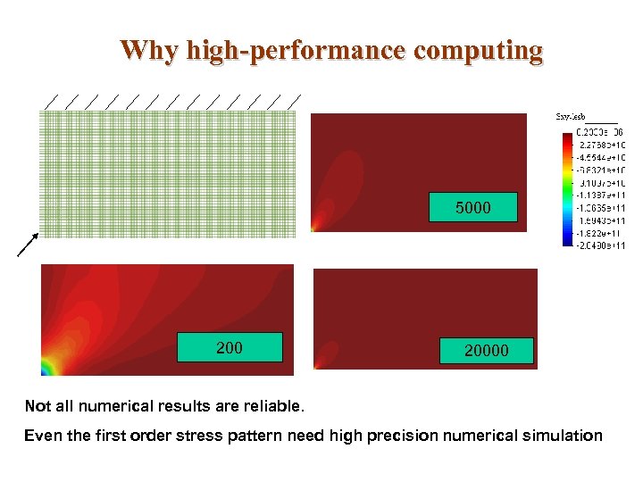
Why high-performance computing 5000 20000 Not all numerical results are reliable. Even the first order stress pattern need high precision numerical simulation

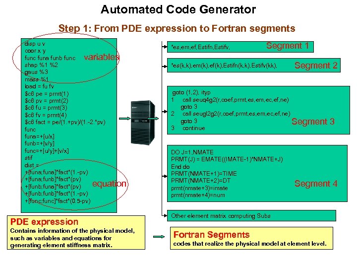
Automated Code Generator Step 1: From PDE expression to Fortran segments disp u v coor x y func funa funb func variables shap %1 %2 gaus %3 mass %1 load = fu fv $c 6 pe = prmt(1) $c 6 pv = prmt(2) $c 6 fu = prmt(3) $c 6 fv = prmt(4) $c 6 fact = pe/(1. +pv)/(1. -2. *pv) func funa=+[u/x] funb=+[v/y] func=+[u/y]+[v/x] stif dist = +[funa; funa]*fact*(1. -pv) +[funa; funb]*fact*(pv) equation +[funb; funa]*fact*(pv) +[funb; funb]*fact*(1. -pv) +[func; func]*fact*(0. 5 -pv) PDE expression Contains information of the physical model, such as variables and equations for generating element stiffness matrix. *es, em, ef, Estifn, Estifv, Segment 1 *es(k, k), em(k), ef(k), Estifn(k, k), Estifv(kk), Segment 2 goto (1, 2), ityp 1 call seuq 4 g 2(r, coef, prmt, es, em, ec, ef, ne) goto 3 2 call seugl 2 g 2(r, coef, prmt, es, em, ec, ef, ne) goto 3 Segment 3 continue DO J=1, NMATE PRMT(J) = EMATE((IMATE-1)*NMATE+J) End do PRMT(NMATE+1)=TIME PRMT(NMATE+2)=DT prmt(nmate+3)=imate prmt(nmate+4)=num 3 Segment 4 Other element matrix computing Subs Fortran Segments codes that realize the physical model at element level.

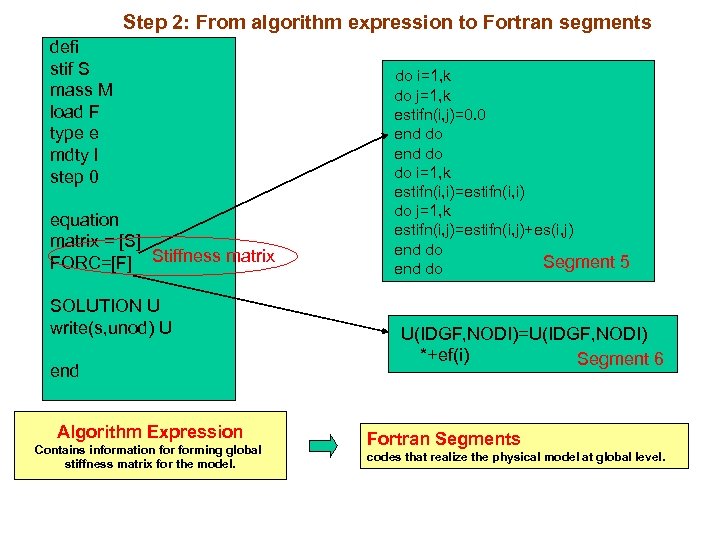
Step 2: From algorithm expression to Fortran segments defi stif S mass M load F type e mdty l step 0 equation matrix = [S] FORC=[F] Stiffness matrix SOLUTION U write(s, unod) U end Algorithm Expression Contains information forming global stiffness matrix for the model. do i=1, k do j=1, k estifn(i, j)=0. 0 end do do i=1, k estifn(i, i)=estifn(i, i) do j=1, k estifn(i, j)=estifn(i, j)+es(i, j) end do Segment 5 end do U(IDGF, NODI)=U(IDGF, NODI) *+ef(i) Segment 6 Fortran Segments codes that realize the physical model at global level.

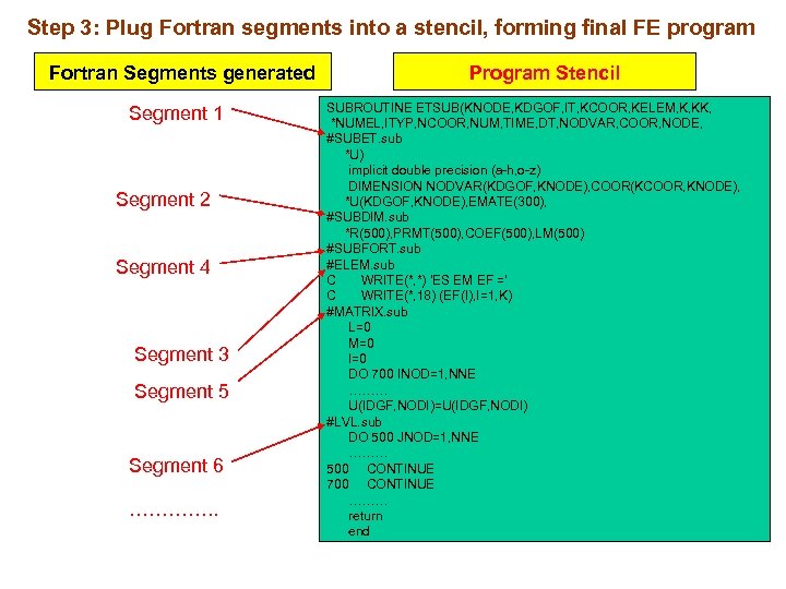
Step 3: Plug Fortran segments into a stencil, forming final FE program Fortran Segments generated Segment 1 Segment 2 Segment 4 Segment 3 Segment 5 Segment 6 …………. . Program Stencil SUBROUTINE ETSUB(KNODE, KDGOF, IT, KCOOR, KELEM, K, KK, *NUMEL, ITYP, NCOOR, NUM, TIME, DT, NODVAR, COOR, NODE, #SUBET. sub *U) implicit double precision (a-h, o-z) DIMENSION NODVAR(KDGOF, KNODE), COOR(KCOOR, KNODE), *U(KDGOF, KNODE), EMATE(300), #SUBDIM. sub *R(500), PRMT(500), COEF(500), LM(500) #SUBFORT. sub #ELEM. sub C WRITE(*, *) 'ES EM EF =' C WRITE(*, 18) (EF(I), I=1, K) #MATRIX. sub L=0 M=0 I=0 DO 700 INOD=1, NNE ……… U(IDGF, NODI)=U(IDGF, NODI) #LVL. sub DO 500 JNOD=1, NNE ……… 500 CONTINUE 700 CONTINUE ……… return end

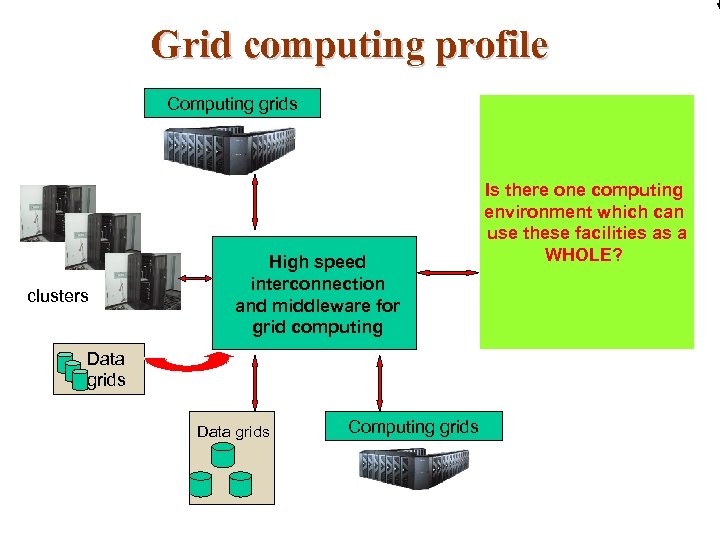
Grid computing profile Computing grids clusters High speed interconnection and middleware for grid computing Data grids Computing grids Is there one computing environment which can use these facilities as a WHOLE?

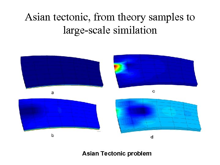
Asian tectonic, from theory samples to large-scale similation Asian Tectonic problem

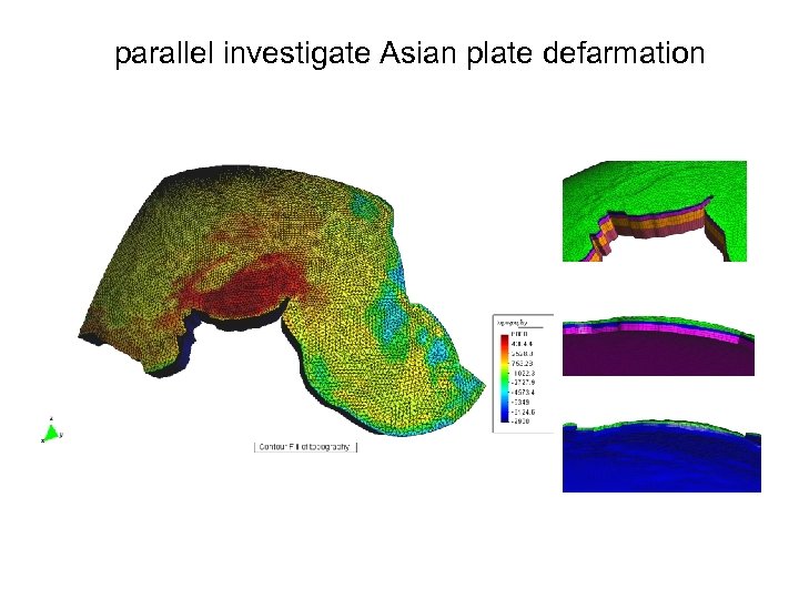
parallel investigate Asian plate defarmation

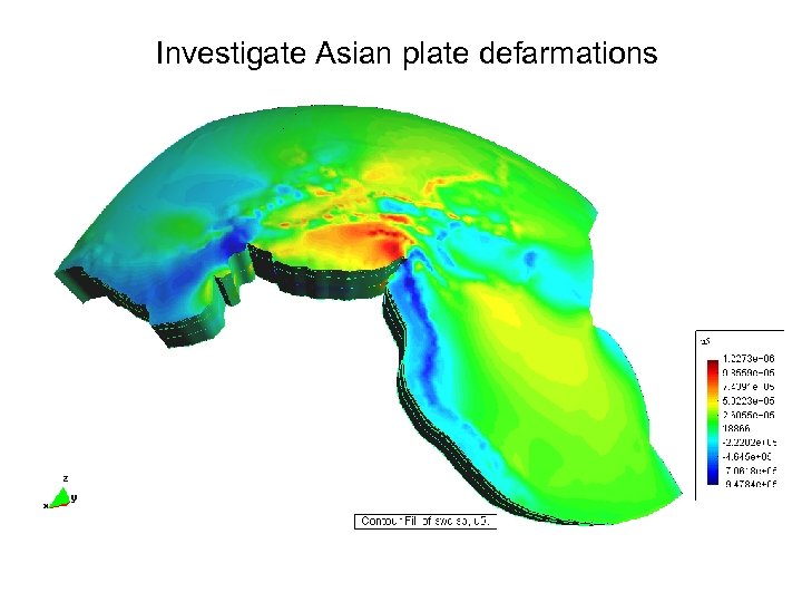
Investigate Asian plate defarmations

Developing full 3 -D model of tsunami

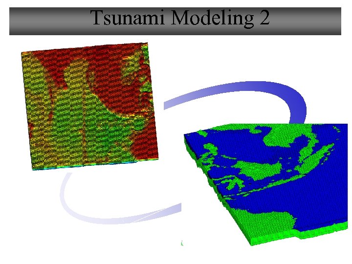
Tsunami Modeling 2

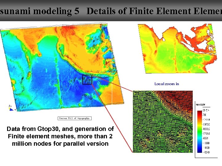
sunami modeling 5 Details of Finite Element Elemen Local zoom in Data from Gtop 30, and generation of Finite element meshes, more than 2 million nodes for parallel version

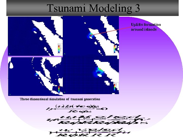
Tsunami Modeling 3 Uplifts formation around islands Three dimensional simulation of tsunami generation

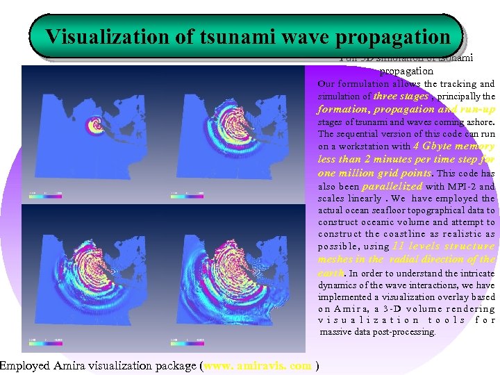
Visualization of tsunami wave propagation Full 3 D simulation of tsunami propagation Our formulation allows the tracking and simulation of three stages , principally the formation, propagation and run-up stages of tsunami and waves coming ashore. The sequential version of this code can run on a workstation with 4 Gbyte memory less than 2 minutes per time step for one million grid points. This code has also been parallelized with MPI-2 and scales linearly. We have employed the actual ocean seafloor topographical data to construct oceanic volume and attempt to construct the coastline as realistic as possible, using 11 levels structure meshes in the radial direction of the earth. In order to understand the intricate dynamics of the wave interactions, we have implemented a visualization overlay based o n A m i r a, a 3 - D v o l u m e r e n d e r i n g v i s u a l i z a t i o n t o o l s f o r massive data post-processing. Employed Amira visualization package (www. amiravis. com )