06903199391bc2b6c1051cd9bc71d076.ppt
- Количество слайдов: 49
 Knowledge discovery & data mining: Classification UCLA CS 240 A Winter 2002 Notes from a tutorial presented @ EDBT 2000 By Fosca Giannotti and Dino Pedreschi Pisa KDD Lab CNUCE-CNR & Univ. Pisa http: //www-kdd. di. unipi. it/ EDBT 2000 tutorial Konstanz, March 2000
 Module outline z The classification task z Main classification techniques y. Bayesian classifiers y. Decision trees y. Hints to other methods z Discussion EDBT 2000 tutorial - Class Konstanz, 27 -28. 3. 2000 2
 The classification task z Input: a training set of tuples, each labelled with one class label z Output: a model (classifier) which assigns a class label to each tuple based on the other attributes. z The model can be used to predict the class of new tuples, for which the class label is missing or unknown z Some natural applications y credit approval y medical diagnosis y treatment effectiveness analysis EDBT 2000 tutorial - Class Konstanz, 27 -28. 3. 2000 3
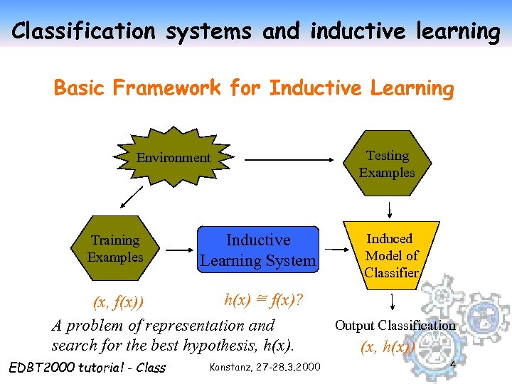 Classification systems and inductive learning Basic Framework for Inductive Learning Environment Training Examples Inductive Learning System ~ h(x) = f(x)? (x, f(x)) A problem of representation and search for the best hypothesis, h(x). EDBT 2000 tutorial - Class Konstanz, 27 -28. 3. 2000 Testing Examples Induced Model of Classifier Output Classification (x, h(x)) 4
 Train & test z The tuples (observations, samples) are partitioned in training set + test set. z Classification is performed in two steps: 1. training - build the model from training set 2. test - check accuracy of the model using test set EDBT 2000 tutorial - Class Konstanz, 27 -28. 3. 2000 5
 Train & test z Kind of models y. IF-THEN rules y. Other logical formulae y. Decision trees z Accuracy of models y. The known class of test samples is matched against the class predicted by the model. y. Accuracy rate = % of test set samples correctly classified by the model. EDBT 2000 tutorial - Class Konstanz, 27 -28. 3. 2000 6
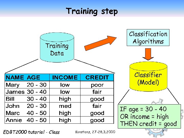 Training step Classification Algorithms Training Data Classifier (Model) IF age = 30 - 40 OR income = high THEN credit = good EDBT 2000 tutorial - Class Konstanz, 27 -28. 3. 2000 7
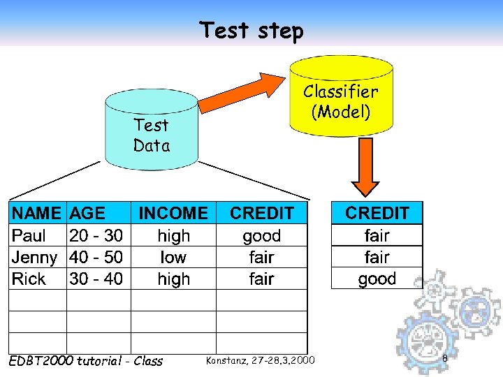 Test step Test Data EDBT 2000 tutorial - Classifier (Model) Konstanz, 27 -28. 3. 2000 8
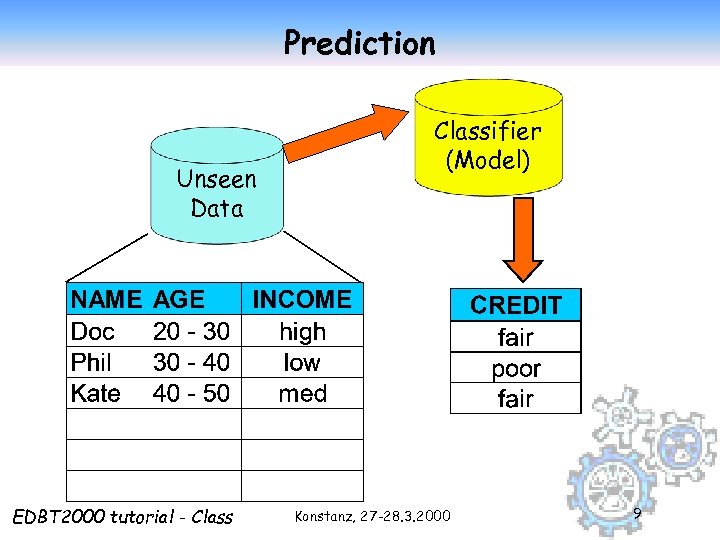 Prediction Unseen Data EDBT 2000 tutorial - Classifier (Model) Konstanz, 27 -28. 3. 2000 9
 Machine learning terminology z Classification = supervised learning yuse training samples with known classes to classify new data z Clustering = unsupervised learning ytraining samples have no class information yguess classes or clusters in the data EDBT 2000 tutorial - Class Konstanz, 27 -28. 3. 2000 10
 Comparing classifiers z Accuracy z Speed z Robustness y w. r. t. noise and missing values z Scalability y efficiency in large databases z Interpretability of the model z Simplicity y decision tree size y rule compactness z Domain-dependent quality indicators EDBT 2000 tutorial - Class Konstanz, 27 -28. 3. 2000 11
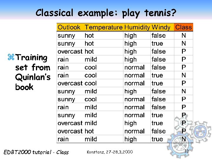 Classical example: play tennis? z Training set from Quinlan’s book EDBT 2000 tutorial - Class Konstanz, 27 -28. 3. 2000 12
 Module outline z The classification task z Main classification techniques y. Bayesian classifiers y. Decision trees y. Hints to other methods z Application to a case-study in fraud detection: planning of fiscal audits EDBT 2000 tutorial - Class Konstanz, 27 -28. 3. 2000 13
 Bayesian classification z The classification problem may be formalized using a-posteriori probabilities: z P(C|X) = prob. that the sample tuple X=
 Estimating a-posteriori probabilities z Bayes theorem: P(C|X) = P(X|C)·P(C) / P(X) z P(X) is constant for all classes z P(C) = relative freq of class C samples z C such that P(C|X) is maximum = C such that P(X|C)·P(C) is maximum z Problem: computing P(X|C) is unfeasible! EDBT 2000 tutorial - Class Konstanz, 27 -28. 3. 2000 15
 Naïve Bayesian Classification z Naïve assumption: attribute independence P(x 1, …, xk|C) = P(x 1|C)·…·P(xk|C) z If i-th attribute is categorical: P(xi|C) is estimated as the relative freq of samples having value xi as i-th attribute in class C z If i-th attribute is continuous: P(xi|C) is estimated thru a Gaussian density function z Computationally easy in both cases EDBT 2000 tutorial - Class Konstanz, 27 -28. 3. 2000 16
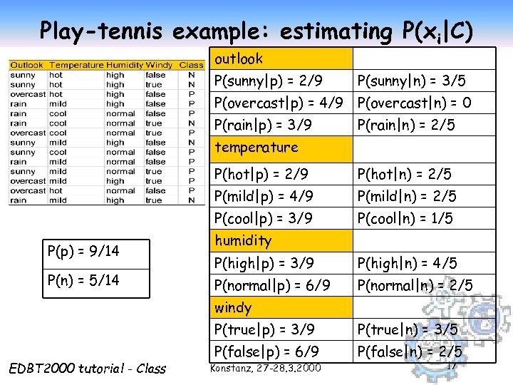 Play-tennis example: estimating P(xi|C) outlook P(sunny|p) = 2/9 P(sunny|n) = 3/5 P(overcast|p) = 4/9 P(overcast|n) = 0 P(rain|p) = 3/9 P(rain|n) = 2/5 temperature P(hot|p) = 2/9 P(mild|p) = 4/9 P(n) = 5/14 P(mild|n) = 2/5 P(cool|p) = 3/9 P(p) = 9/14 P(hot|n) = 2/5 P(cool|n) = 1/5 humidity P(high|p) = 3/9 P(high|n) = 4/5 P(normal|p) = 6/9 P(normal|n) = 2/5 windy P(true|p) = 3/9 EDBT 2000 tutorial - Class P(true|n) = 3/5 P(false|p) = 6/9 P(false|n) = 2/5 Konstanz, 27 -28. 3. 2000 17
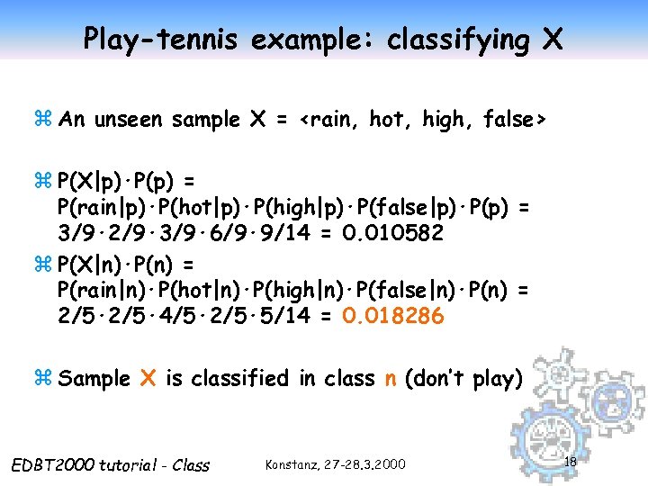 Play-tennis example: classifying X z An unseen sample X =
 The independence hypothesis… z … makes computation possible z … yields optimal classifiers when satisfied z … but is seldom satisfied in practice, as attributes (variables) are often correlated. z Attempts to overcome this limitation: y. Bayesian networks, that combine Bayesian reasoning with causal relationships between attributes y. Decision trees, that reason on one attribute at the time, considering most important attributes first EDBT 2000 tutorial - Class Konstanz, 27 -28. 3. 2000 19
 Module outline z The classification task z Main classification techniques y. Bayesian classifiers y. Decision trees y. Hints to other methods EDBT 2000 tutorial - Class Konstanz, 27 -28. 3. 2000 20
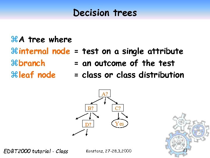 Decision trees z A tree where z internal node = test on a single attribute z branch = an outcome of the test z leaf node = class or class distribution A? B? D? EDBT 2000 tutorial - Class C? Yes Konstanz, 27 -28. 3. 2000 21
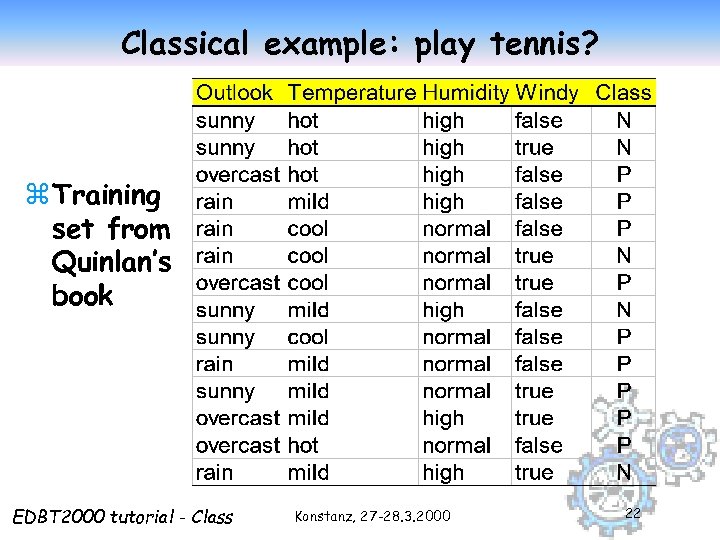 Classical example: play tennis? z Training set from Quinlan’s book EDBT 2000 tutorial - Class Konstanz, 27 -28. 3. 2000 22
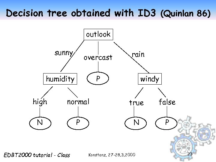 Decision tree obtained with ID 3 (Quinlan 86) outlook sunny overcast humidity rain windy P high normal true false N P EDBT 2000 tutorial - Class Konstanz, 27 -28. 3. 2000 23
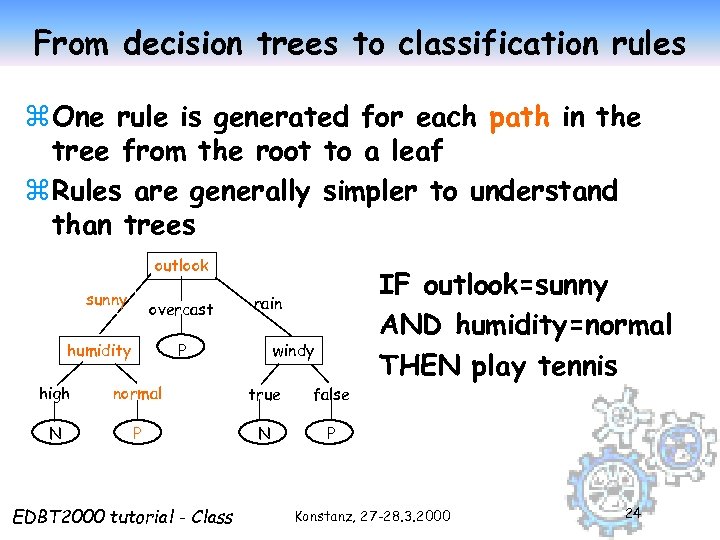 From decision trees to classification rules z One rule is generated for each path in the tree from the root to a leaf z Rules are generally simpler to understand than trees outlook sunny overcast humidity rain windy P high normal true false N P N IF outlook=sunny AND humidity=normal THEN play tennis P EDBT 2000 tutorial - Class Konstanz, 27 -28. 3. 2000 24
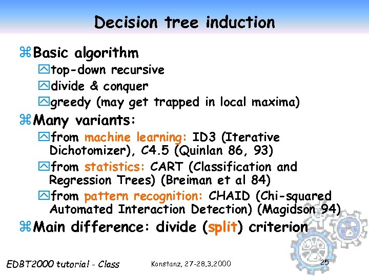 Decision tree induction z Basic algorithm ytop-down recursive ydivide & conquer ygreedy (may get trapped in local maxima) z Many variants: yfrom machine learning: ID 3 (Iterative Dichotomizer), C 4. 5 (Quinlan 86, 93) yfrom statistics: CART (Classification and Regression Trees) (Breiman et al 84) yfrom pattern recognition: CHAID (Chi-squared Automated Interaction Detection) (Magidson 94) z Main difference: divide (split) criterion EDBT 2000 tutorial - Class Konstanz, 27 -28. 3. 2000 25
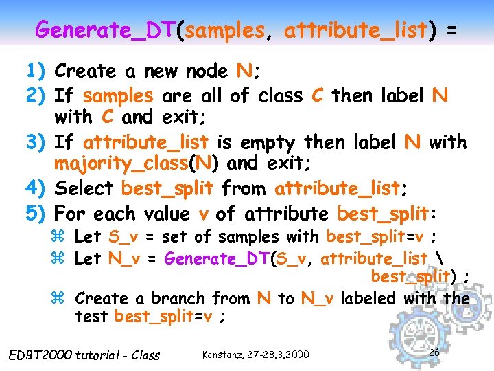 Generate_DT(samples, attribute_list) = 1) Create a new node N; 2) If samples are all of class C then label N with C and exit; 3) If attribute_list is empty then label N with majority_class(N) and exit; 4) Select best_split from attribute_list; 5) For each value v of attribute best_split: z Let S_v = set of samples with best_split=v ; z Let N_v = Generate_DT(S_v, attribute_list best_split) ; z Create a branch from N to N_v labeled with the test best_split=v ; EDBT 2000 tutorial - Class Konstanz, 27 -28. 3. 2000 26
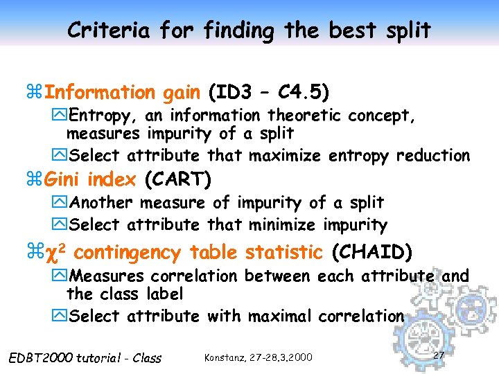 Criteria for finding the best split z Information gain (ID 3 – C 4. 5) y. Entropy, an information theoretic concept, measures impurity of a split y. Select attribute that maximize entropy reduction z Gini index (CART) y. Another measure of impurity of a split y. Select attribute that minimize impurity z 2 contingency table statistic (CHAID) y. Measures correlation between each attribute and the class label y. Select attribute with maximal correlation EDBT 2000 tutorial - Class Konstanz, 27 -28. 3. 2000 27
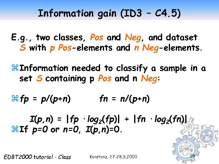 Information gain (ID 3 – C 4. 5) E. g. , two classes, Pos and Neg, and dataset S with p Pos-elements and n Neg-elements. z Information needed to classify a sample in a set S containing p Pos and n Neg: z fp = p/(p+n) fn = n/(p+n) I(p, n) = |fp ·log 2(fp)| + |fn ·log 2(fn)| z If p=0 or n=0, I(p, n)=0. EDBT 2000 tutorial - Class Konstanz, 27 -28. 3. 2000 28
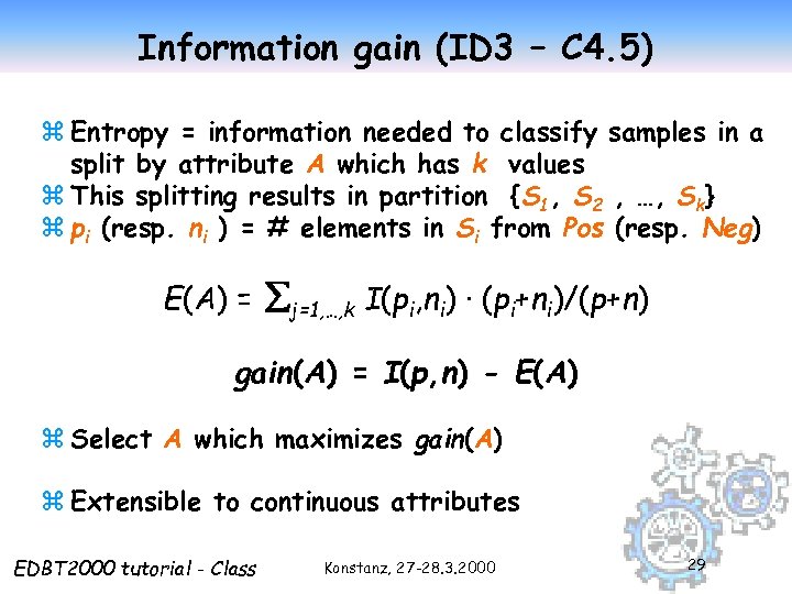 Information gain (ID 3 – C 4. 5) z Entropy = information needed to classify samples in a split by attribute A which has k values z This splitting results in partition {S 1, S 2 , …, Sk} z pi (resp. ni ) = # elements in Si from Pos (resp. Neg) E(A) = j=1, …, k I(pi, ni) · (pi+ni)/(p+n) gain(A) = I(p, n) - E(A) z Select A which maximizes gain(A) z Extensible to continuous attributes EDBT 2000 tutorial - Class Konstanz, 27 -28. 3. 2000 29
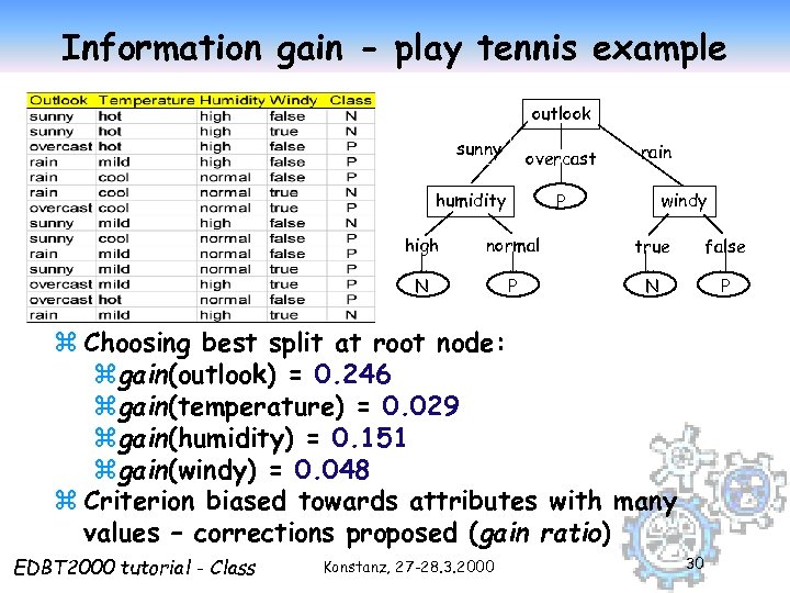 Information gain - play tennis example outlook sunny overcast humidity rain windy P high normal true false N P z Choosing best split at root node: zgain(outlook) = 0. 246 zgain(temperature) = 0. 029 zgain(humidity) = 0. 151 zgain(windy) = 0. 048 z Criterion biased towards attributes with many values – corrections proposed (gain ratio) EDBT 2000 tutorial - Class Konstanz, 27 -28. 3. 2000 30
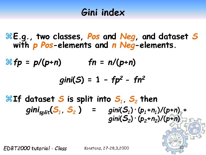 Gini index z E. g. , two classes, Pos and Neg, and dataset S with p Pos-elements and n Neg-elements. z fp = p/(p+n) fn = n/(p+n) gini(S) = 1 – fp 2 - fn 2 z If dataset S is split into S 1, S 2 then ginisplit(S 1, S 2 ) = gini(S 1)·(p 1+n 1)/(p+n) + gini(S 2)·(p 2+n 2)/(p+n) EDBT 2000 tutorial - Class Konstanz, 27 -28. 3. 2000 31
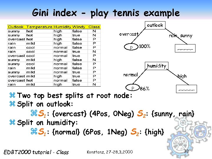 Gini index - play tennis example outlook overcast P rain, sunny 100% …………… humidity normal P high 86% …………… z Two top best splits at root node: z Split on outlook: z. S 1: {overcast} (4 Pos, 0 Neg) S 2: {sunny, rain} z Split on humidity: z. S 1: {normal} (6 Pos, 1 Neg) S 2: {high} EDBT 2000 tutorial - Class Konstanz, 27 -28. 3. 2000 32
 Other criteria in decision tree construction z Branching scheme: ybinary vs. k-ary splits ycategorical vs. continuous attributes z Stop rule: how to decide that a node is a leaf: y all samples belong to same class y impurity measure below a given threshold y no more attributes to split on y no samples in partition z Labeling rule: a leaf node is labeled with the class to which most samples at the node belong EDBT 2000 tutorial - Class Konstanz, 27 -28. 3. 2000 33
 The overfitting problem z Ideal goal of classification: find the simplest decision tree that fits the data and generalizes to unseen data y intractable in general z A decision tree may become too complex if it overfits the training samples, due to y noise and outliers, or y too little training data, or y local maxima in the greedy search z Two heuristics to avoid overfitting: y. Stop earlier: Stop growing the tree earlier. y. Post-prune: Allow overfit, and then simplify the tree. EDBT 2000 tutorial - Class Konstanz, 27 -28. 3. 2000 34
 Stopping vs. pruning z Stopping: Prevent the split on an attribute (predictor variable) if it is below a level of statistical significance - simply make it a leaf (CHAID) z Pruning: After a complex tree has been grown, replace a split (subtree) with a leaf if the predicted validation error is no worse than the more complex tree (CART, C 4. 5) z Integration of the two: PUBLIC (Rastogi and Shim 98) – estimate pruning conditions (lower bound to minimum cost subtrees) during construction, and use them to stop. EDBT 2000 tutorial - Class Konstanz, 27 -28. 3. 2000 35
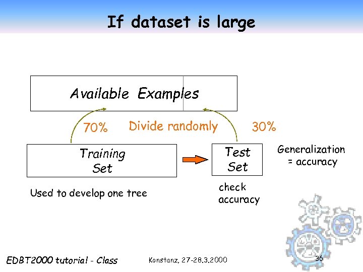 If dataset is large Available Examples 70% Divide randomly Training Set Used to develop one tree EDBT 2000 tutorial - Class 30% Test Set Generalization = accuracy check accuracy Konstanz, 27 -28. 3. 2000 36
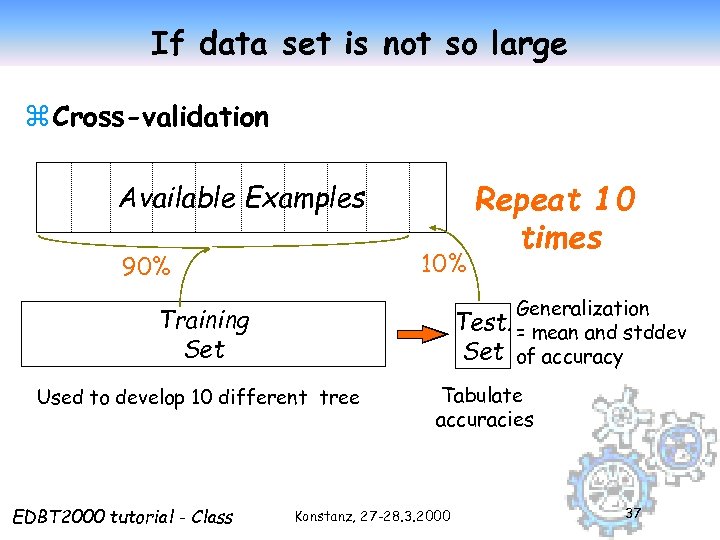 If data set is not so large z Cross-validation Available Examples 10% 90% Generalization Test. = mean and stddev Set of accuracy Training Set Used to develop 10 different tree EDBT 2000 tutorial - Class Repeat 10 times Tabulate accuracies Konstanz, 27 -28. 3. 2000 37
 Categorical vs. continuous attributes z Information gain criterion may be adapted to continuous attributes using binary splits z Gini index may be adapted to categorical. z Typically, discretization is not a preprocessing step, but is performed dynamically during the decision tree construction. EDBT 2000 tutorial - Class Konstanz, 27 -28. 3. 2000 38
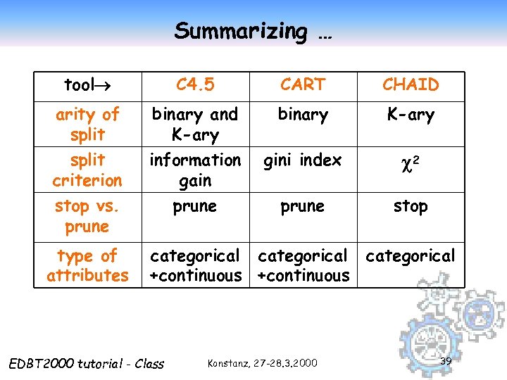 Summarizing … tool C 4. 5 CART CHAID arity of split binary and K-ary binary K-ary split criterion information gain gini index 2 stop vs. prune stop type of attributes categorical +continuous EDBT 2000 tutorial - Class Konstanz, 27 -28. 3. 2000 39
 Scalability to large databases z What if the dataset does not fit main memory? z Early approaches: y Incremental tree construction (Quinlan 86) y Merge of trees constructed on separate data partitions (Chan & Stolfo 93) y Data reduction via sampling (Cattlet 91) z Goal: handle order of 1 G samples and 1 K attributes z Successful contributions from data mining research y SLIQ (Mehta et al. 96) y SPRINT y PUBLIC y Rain. Forest (Shafer et al. 96) (Rastogi & Shim 98) EDBT 2000 tutorial - Class (Gehrke et al. 98) Konstanz, 27 -28. 3. 2000 40
 Classification with decision trees z Reference technique: y. Quinlan’s C 4. 5, and its evolution C 5. 0 z Advanced mechanisms used: ypruning factor ymisclassification weights yboosting factor EDBT 2000 tutorial - Class Konstanz, 27 -28. 3. 2000 41
 Bagging and Boosting z Bagging: build a set of classifiers from different samples of the same trainingset. Decision by voting. z Boosting: assign more weight to missclassied tuples. Can be used to build the n+1 classifier, or to improve the old one. EDBT 2000 tutorial - Class Konstanz, 27 -28. 3. 2000 42
 Module outline z The classification task z Main classification techniques y. Decision trees y. Bayesian classifiers y. Hints to other methods EDBT 2000 tutorial - Class Konstanz, 27 -28. 3. 2000 43
 Backpropagation z Is a neural network algorithm, performing on multilayer feed-forward networks (Rumelhart et al. 86). z A network is a set of connected input/output units where each connection has an associated weight. z The weights are adjusted during the training phase, in order to correctly predict the class label for samples. EDBT 2000 tutorial - Class Konstanz, 27 -28. 3. 2000 44
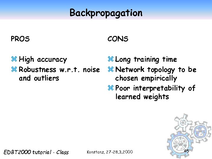 Backpropagation PROS CONS z High accuracy z Robustness w. r. t. noise and outliers z Long training time z Network topology to be chosen empirically z Poor interpretability of learned weights EDBT 2000 tutorial - Class Konstanz, 27 -28. 3. 2000 45
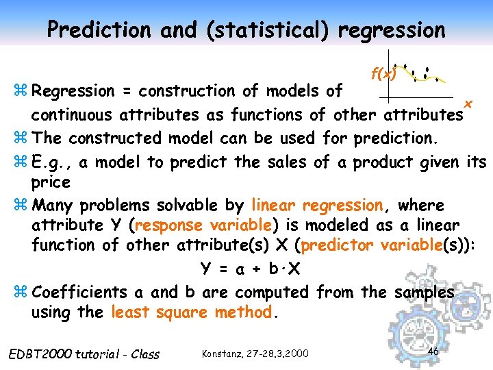 Prediction and (statistical) regression f(x) z Regression = construction of models of x continuous attributes as functions of other attributes z The constructed model can be used for prediction. z E. g. , a model to predict the sales of a product given its price z Many problems solvable by linear regression, where attribute Y (response variable) is modeled as a linear function of other attribute(s) X (predictor variable(s)): Y = a + b·X z Coefficients a and b are computed from the samples using the least square method. EDBT 2000 tutorial - Class Konstanz, 27 -28. 3. 2000 46
 Other methods (not covered) z K-nearest neighbors algorithms z Case-based reasoning z Genetic algorithms z Rough sets z Fuzzy logic z Association-based classification (Liu et al 98) EDBT 2000 tutorial - Class Konstanz, 27 -28. 3. 2000 47
 References - classification z C. Apte and S. Weiss. Data mining with decision trees and decision rules. Future Generation Computer Systems, 13, 1997. z F. Bonchi, F. Giannotti, G. Mainetto, D. Pedreschi. Using Data Mining Techniques in Fiscal Fraud Detection. In Proc. Da. Wak'99, First Int. Conf. on Data Warehousing and Knowledge Discovery, Sept. 1999. z F. Bonchi , F. Giannotti, G. Mainetto, D. Pedreschi. A Classification-based Methodology for Planning Audit Strategies in Fraud Detection. In Proc. KDD-99, ACM-SIGKDD Int. Conf. on Knowledge Discovery & Data Mining, Aug. 1999. z z J. Catlett. Megainduction: machine learning on very large databases. Ph. D Thesis, Univ. Sydney, 1991. z z z J. R. Quinlan. C 4. 5: Programs for Machine Learning. Morgan Kaufman, 1993. z P. K. Chan and S. J. Stolfo. Learning arbiter and combiner trees from partitioned data for scaling machine learning. In Proc. KDD'95, August 1995. z J. Gehrke, R. Ramakrishnan, and V. Ganti. Rainforest: A framework for fast decision tree construction of large datasets. In Proc. 1998 Int. Conf. Very Large Data Bases, pages 416 -427, New York, NY, August 1998. z B. Liu, W. Hsu and Y. Ma. Integrating classification and association rule mining. In Proc. KDD’ 98, New York, 1998. P. K. Chan and S. J. Stolfo. Metalearning for multistrategy and parallel learning. In Proc. 2 nd Int. Conf. on Information and Knowledge Management, p. 314 -323, 1993. J. R. Quinlan. Induction of decision trees. Machine Learning, 1: 81 -106, 1986. L. Breiman, J. Friedman, R. Olshen, and C. Stone. Classification and Regression Trees. Wadsworth International Group, 1984. EDBT 2000 tutorial - Class Konstanz, 27 -28. 3. 2000 48
 References - classification z z z z J. Magidson. The CHAID approach to segmentation modeling: Chi-squared automatic interaction detection. In R. P. Bagozzi, editor, Advanced Methods of Marketing Research, pages 118 -159. Blackwell Business, Cambridge Massechusetts, 1994. M. Mehta, R. Agrawal, and J. Rissanen. SLIQ : A fast scalable classifier for data mining. In Proc. 1996 Int. Conf. Extending Database Technology (EDBT'96), Avignon, France, March 1996. S. K. Murthy, Automatic Construction of Decision Trees from Data: A Multi-Diciplinary Survey. Data Mining and Knowledge Discovery 2(4): 345 -389, 1998 J. R. Quinlan. Bagging, boosting, and C 4. 5. In Proc. 13 th Natl. Conf. on Artificial Intelligence (AAAI'96), 725 -730, Portland, OR, Aug. 1996. R. Rastogi and K. Shim. Public: A decision tree classifer that integrates building and pruning. In Proc. 1998 Int. Conf. Very Large Data Bases, 404 -415, New York, NY, August 1998. J. Shafer, R. Agrawal, and M. Mehta. SPRINT : A scalable parallel classifier for data mining. In Proc. 1996 Int. Conf. Very Large Data Bases, 544 -555, Bombay, India, Sept. 1996. S. M. Weiss and C. A. Kulikowski. Computer Systems that Learn: Classification and Prediction Methods from Statistics, Neural Nets, Machine Learning, and Expert Systems. Morgan Kaufman, 1991. D. E. Rumelhart, G. E. Hinton and R. J. Williams. Learning internal representation by error propagation. In D. E. Rumelhart and J. L. Mc. Clelland (eds. ) Parallel Distributed Processing. The MIT Press, 1986 EDBT 2000 tutorial - Class Konstanz, 27 -28. 3. 2000 49


