fd3d6b90861195f472482f71a2614ad0.ppt
- Количество слайдов: 35

July 5 th 2006 Object Recognition using Local Invariant Features Claudio Scordino scordino@di. unipi. it
Object Recognition n Widely used in the industry for n n n Current commercial systems n n Inspection Registration Manipulation Robot localization and mapping Correlation-based template matching Computationally infeasible when object rotation, scale, illumination and 3 D pose vary Even more infeasible with partial occlusion Alternative: Local Image Features
Local Image Features n Unaffected by n n n Nearby clutter Partial occlusion Invariant to n n 3 D projective transforms n n Illumination Common object variations . . . but, at the same time, sufficiently distinctive to identify specific objects among many alternatives!
Related work n Line segments, edges and regions grouping n n Peaks detection in local image variations n n Detection not good enough for reliable recognition Example: Harris corner detector Drawback: image examined at only a single scale Different key locations as the image scale changes Eigenspace matching, color and receptive field histograms n n Successful on isolated objects Unextendable to cluttered and partially occluded images
SIFT Method n Scale Invariant Feature Transform (SIFT) n Staged filtering approach n n Identifies stable points (image “keys”) Computation time less than 2 secs
SIFT Method (2) n Local features: n Invariant to image translation, scaling, rotation n Partially invariant to illumination changes and 3 D projection (up to 20° of rotation) n Minimally affected by noise n Similar properties with neurons in Inferior Temporal cortex used for object recognition in primate vision
First stage n Input: original image (512 x 512 pixel) n Goal: key localization and image description n Output: SIFT keys n Feature vector describing the local image region sampled relative to its scale-space coordinate frame
First stage (2) n Description: n n Represents blurred image gradient locations in multiple orientations planes and at multiple scales Approach based on a model of cells in the celebral cortex of mammalian vision Less than 1 sec of computation time Build a pyramid of images n n Images are difference-of-Gaussian (DOG) functions Resampling between each level
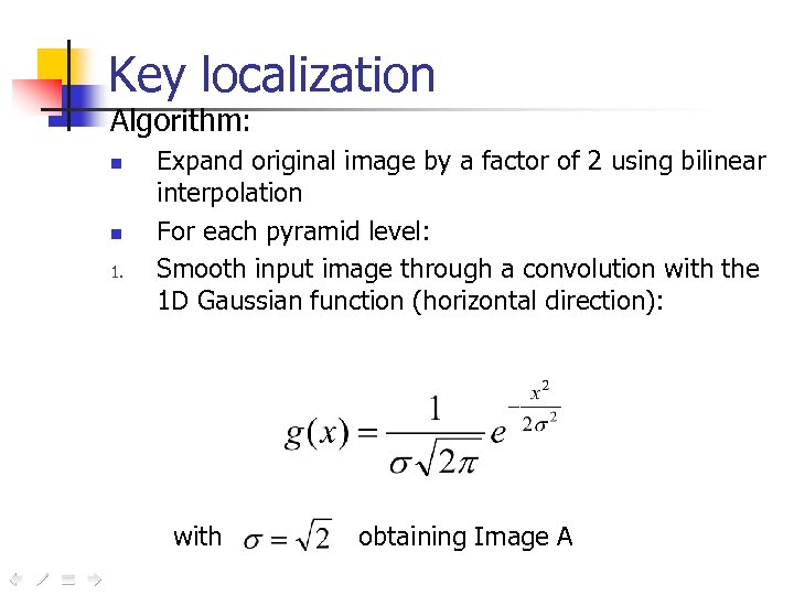
Key localization Algorithm: n n 1. Expand original image by a factor of 2 using bilinear interpolation For each pyramid level: Smooth input image through a convolution with the 1 D Gaussian function (horizontal direction): with obtaining Image A
Key localization (2) Smooth Image A through a further convolution with th 1 D Gaussian function (vertical direction) obtaining Image B 2. The DOG image of this level is B-A 3. Resample Image B using bilinear interpolation with pixel spacing 1. 5 in each direction and use the result as Input Image of the new pyramid level 4. n Each new sample is a constant linear combination of 4 adjacent pixels
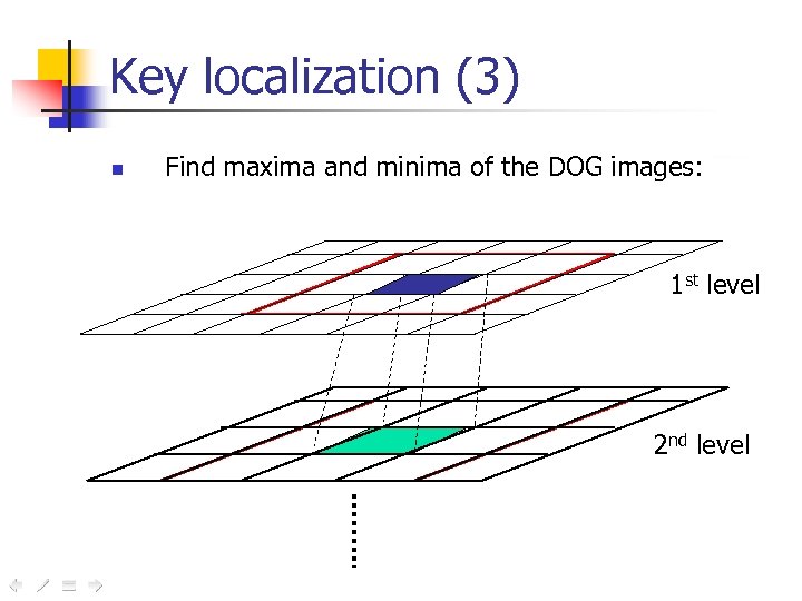
Key localization (3) n Find maxima and minima of the DOG images: 1 st level 2 nd level
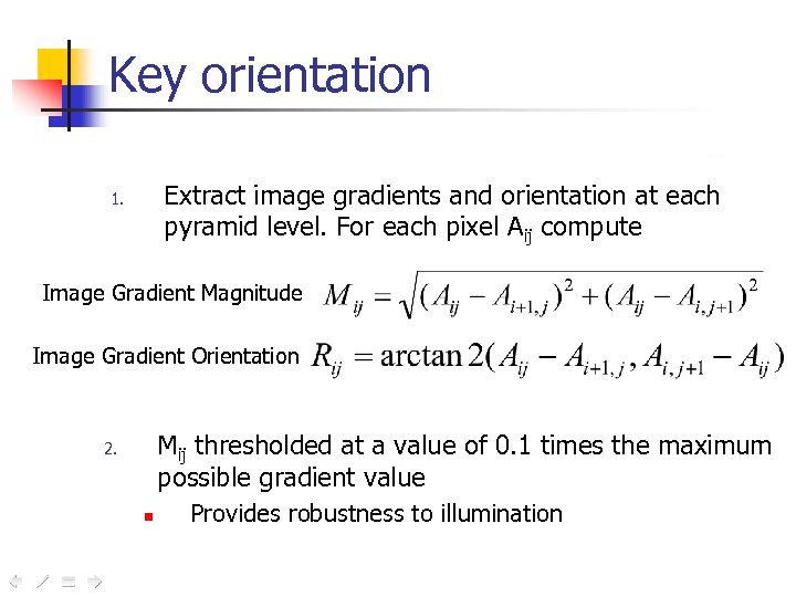
Key orientation Extract image gradients and orientation at each pyramid level. For each pixel Aij compute 1. Image Gradient Magnitude Image Gradient Orientation Mij thresholded at a value of 0. 1 times the maximum possible gradient value 2. n Provides robustness to illumination
Key orientation (2) Create an orientation histogram using a circular Gaussian-weighted window with σ=3 times the current smoothing scale 3. n n n The weights are multiplied by Mij The histogram is smoothed prior to peak selection The orientation is determined by the peak in the histogram
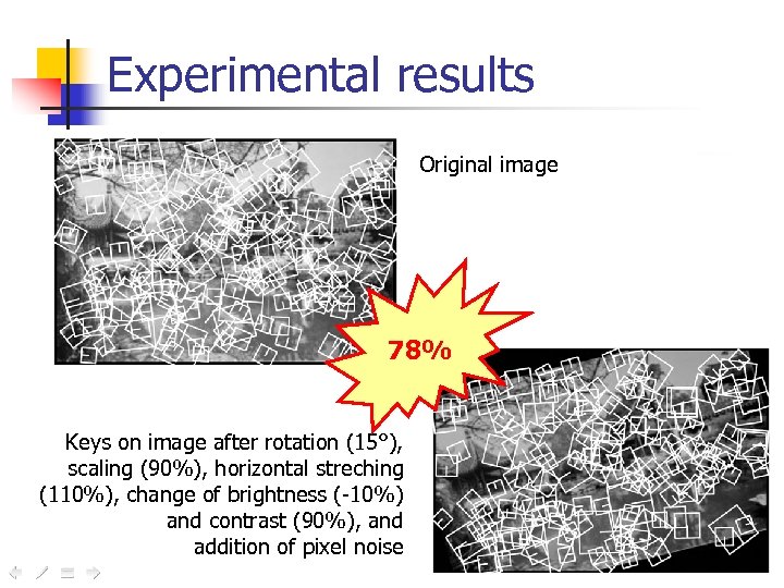
Experimental results Original image 78% Keys on image after rotation (15°), scaling (90%), horizontal streching (110%), change of brightness (-10%) and contrast (90%), and addition of pixel noise
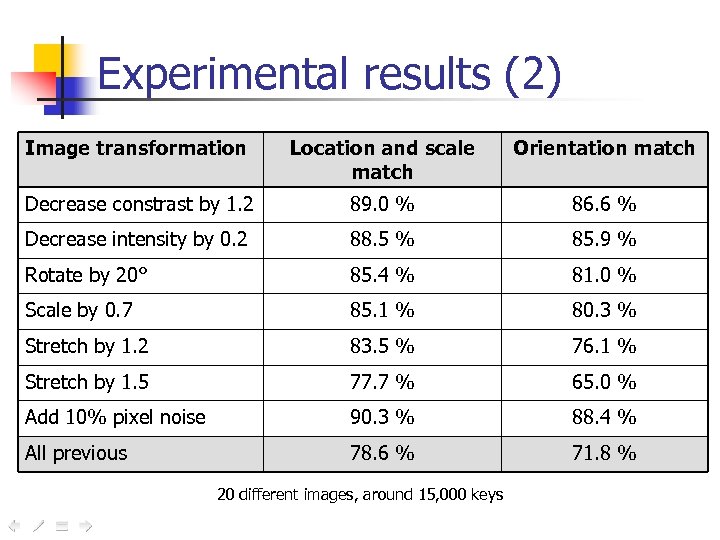
Experimental results (2) Image transformation Location and scale match Orientation match Decrease constrast by 1. 2 89. 0 % 86. 6 % Decrease intensity by 0. 2 88. 5 % 85. 9 % Rotate by 20° 85. 4 % 81. 0 % Scale by 0. 7 85. 1 % 80. 3 % Stretch by 1. 2 83. 5 % 76. 1 % Stretch by 1. 5 77. 7 % 65. 0 % Add 10% pixel noise 90. 3 % 88. 4 % All previous 78. 6 % 71. 8 % 20 different images, around 15, 000 keys
Image description Approach suggested by the response properties of complex neurons in the visual cortex n n A feature position is allowed to vary over a small region, while orientation and spatial frequency are maintained Image descripted through 8 orientation planes n n Keys inserted according to their orientations
Second stage Goal: identify candidate object matches n n n The best candidate match is the nearest neighbour (i. e. , minimum Euclidean distance between decriptor vectors) The exact solution for high dimensional vectors is known to have high complexity
Second stage (2) Algorithm: approximate Best-Bin-First (BBF) search method (Beis and Lowe) n n Modification of the k-d tree algorithm Identifies the nearest neighbours with high probability and small computation The keys generated at the larger scale are given twice the weight of those at the smaller scale n Improves recognition by giving more weight to the leastnoisy scale
Third stage n Description: final verification n Algorithm: low-residual least-squares fit n n n Solution of a linear system: x = [ATA]-1 ATb When at least 3 keys agree with low residual, there is strong evidence for the presence of the object Since there are dozens of keys in the image, this works also with partial occlusion
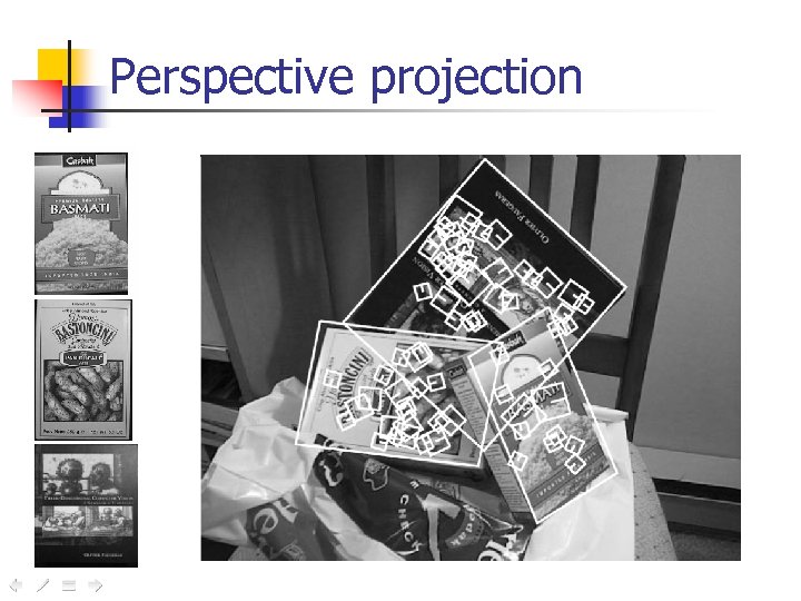
Perspective projection
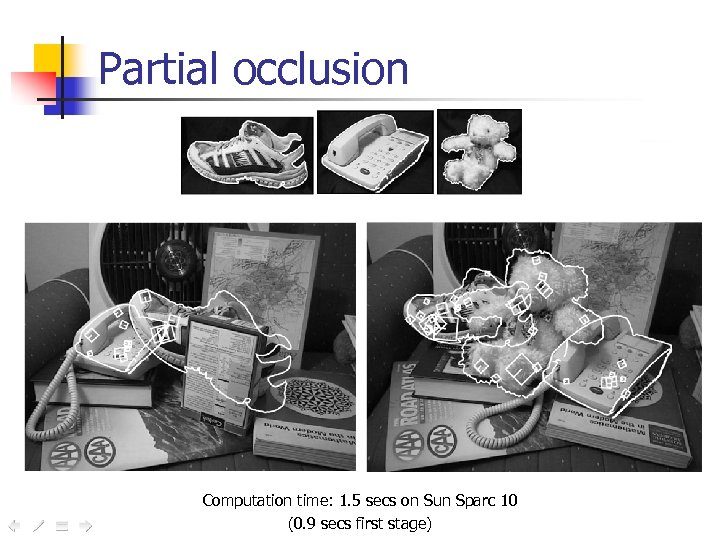
Partial occlusion Computation time: 1. 5 secs on Sun Sparc 10 (0. 9 secs first stage)
Connections to human vision n n Performance of human vision is obviously far superior than current computer vision. . . The brain uses a highly computationalintensive parallel process instead of a staged filtering approach
Connections to human vision However. . . the results are much the same Recent research in neuroscience showed that the neurons of Inferior Temporal cortex n n n Recognize shape features The complexity of the features is roughly the same as for SIFT They also recognize color and texture properties in addition to shape Further research: n n n 3 D structure of objects Additional feature types for color and texture
Augmented Reality (AR) Registration of virtual objects into a live video sequence n Current AR systems: n n n Rely on markers strategically placed in the environment Need manual camera calibration
Related work Harris corner detector and Kanade-Lucas. Tomasi (KLT) tracker n n Parallelogram-shaped and elliptical image regions tracking n n Requires planar structures in viewed scene Pre-built user-supplied CAD object models n n Not enough feature invariance Not always available Limited to objects that can be easily modelled Off-line batch processing of the entire video
AR using SIFT Flexible automated AR Not needed: n n n n n Camera pre-calibration Prior knowledge of scene geometry Manual initialization of the tracker Placement of special markers Special tools or equipment (just a camera) Short time and small effort to setup Robust 6 degrees of freedom
AR using SIFT (2) Need only a set of reference images taken by a handheld uncalibrated camera from arbitrary viewpoints n n n Acquired from unknown spatially separated viewpoints by a handheld camera At least two images n n 5 to 20 images separated by at most 45° Used to build a 3 D model of the viewed scene
AR using SIFT (3) First (off-line) stage: n 1. 2. 3. 4. 5. Extract SIFT features from reference images Establish multi-view correspondences Build a metric model of the real world Compute calibration parameters and camera poses The user places the virtual object n n n The placement is achieved by anchoring object projection in the first image Then, a second projection is adjusted in the second image Finally, the user fine-tunes position, orientation and size
AR using SIFT (4) Second (on-line) stage: n 1. 2. 3. 4. Features are detected in the current frame Features are matched to those of the model using the BBF algorithm The matches are used to compute the current pose of the camera Solution is stabilized by using the values computed for the previous frame
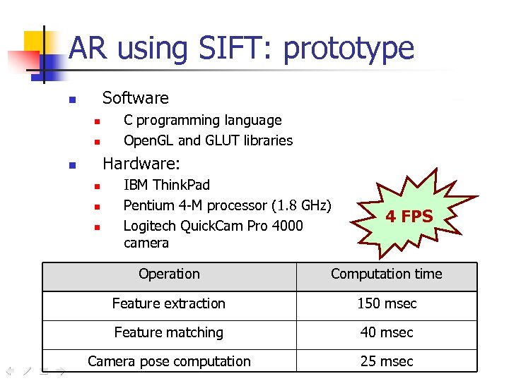
AR using SIFT: prototype Software n n n C programming language Open. GL and GLUT libraries Hardware: n n IBM Think. Pad Pentium 4 -M processor (1. 8 GHz) Logitech Quick. Cam Pro 4000 camera 4 FPS Operation Computation time Feature extraction 150 msec Feature matching 40 msec Camera pose computation 25 msec
AR using SIFT: drawbacks The tracker is very slow n n 4 FPS (Frame Per Second) Too slow for real-time operations (25 FPS) The main bottleneck is feature extraction Unable to handle occlusion of inserted virtual content by real objects n n A full model of the observed scene is required
AR using SIFT: examples Videos: n n n mug tabletop
Conclusions Object recognition using SIFT n n n Reliable recognition Several characteristics in common with human vision Augmented reality using SIFT n n Very flexible Not possible in real-time due to the high computation times In future possible using faster processors
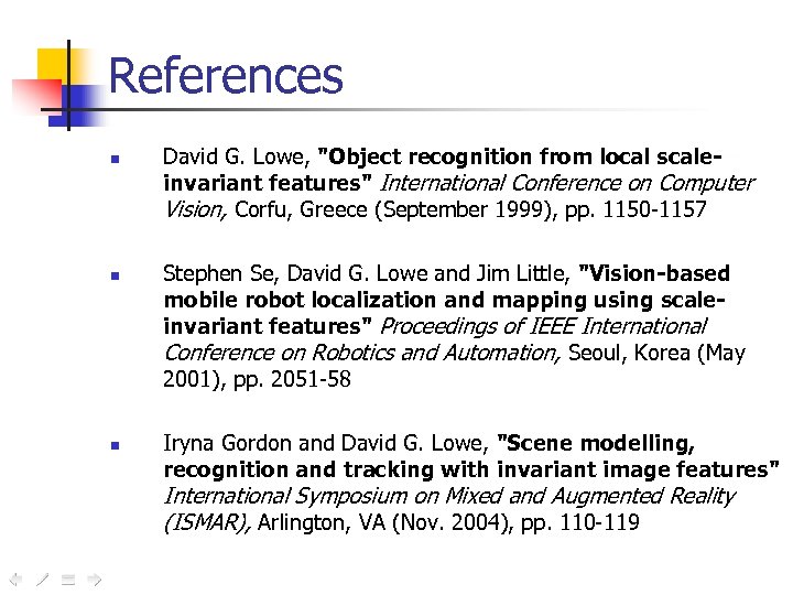
References n n n David G. Lowe, "Object recognition from local scaleinvariant features" International Conference on Computer Vision, Corfu, Greece (September 1999), pp. 1150 -1157 Stephen Se, David G. Lowe and Jim Little, "Vision-based mobile robot localization and mapping using scaleinvariant features" Proceedings of IEEE International Conference on Robotics and Automation, Seoul, Korea (May 2001), pp. 2051 -58 Iryna Gordon and David G. Lowe, "Scene modelling, recognition and tracking with invariant image features" International Symposium on Mixed and Augmented Reality (ISMAR), Arlington, VA (Nov. 2004), pp. 110 -119

For any question. . . David Lowe Computer Science Department 2366 Main Mall University of British Columbia Vancouver, B. C. , V 6 T 1 Z 4, Canada E-mail: lowe@cs. ubc. ca
fd3d6b90861195f472482f71a2614ad0.ppt