It Compress An Iterative Semantic Compression Algorithm H

It. Compress: An Iterative Semantic Compression Algorithm H. V. Jagadish U. Michigan Ann Arbor R. T. Ng U. Of British Columbia Vancouver B. C. Ooi A. K. H. Tung Natl’ U. of Singapore 1

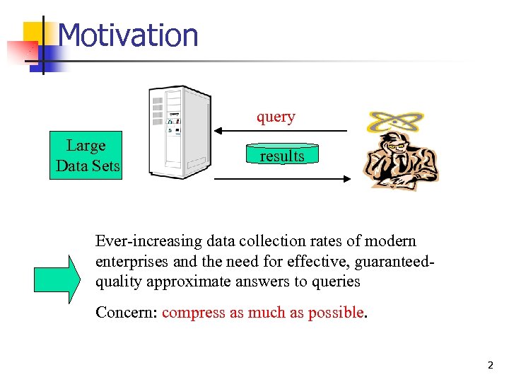Motivation query Large Data Sets results Ever-increasing data collection rates of modern enterprises and the need for effective, guaranteedquality approximate answers to queries Concern: compress as much as possible. 2

Conventional Compression Method n Try to find the optimal encoding of arbitrary strings for the input data: n n n Huffman Coding Lempel-Ziv Coding (gzip) View the whole table as a large byte string Statistical or dictionary based Operate at the byte level 3

Why not just “syntactic”? n n n Do not exploit the complex dependency patterns in the table Individual retrieval of tuple is difficult Do not utilize lossy compression 4

Outline n n n Motivation Semantic Compression Methods It. Compress Algorithm Performance Conclusion Q&A 5

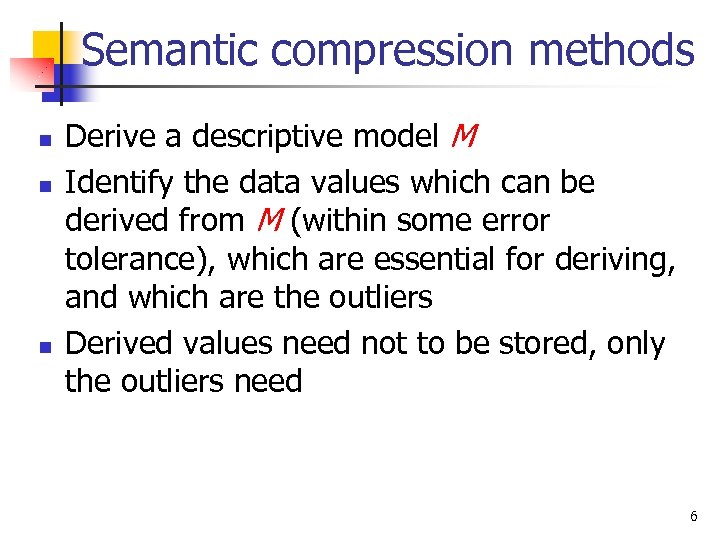Semantic compression methods n n n Derive a descriptive model M Identify the data values which can be derived from M (within some error tolerance), which are essential for deriving, and which are the outliers Derived values need not to be stored, only the outliers need 6

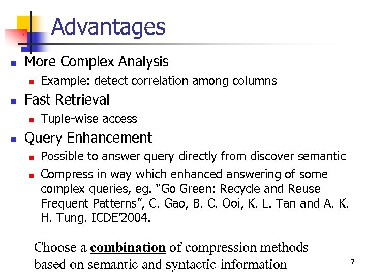Advantages n More Complex Analysis n n Fast Retrieval n n Example: detect correlation among columns Tuple-wise access Query Enhancement n n Possible to answer query directly from discover semantic Compress in way which enhanced answering of some complex queries, eg. “Go Green: Recycle and Reuse Frequent Patterns”, C. Gao, B. C. Ooi, K. L. Tan and A. K. H. Tung. ICDE’ 2004. Choose a combination of compression methods based on semantic and syntactic information 7

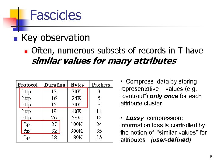Fascicles n Key observation n Often, numerous subsets of records in T have similar values for many attributes Protocol http http ftp ftp Duration Bytes 12 20 K 16 24 K 15 20 K 19 40 K 26 58 K 27 100 K 32 300 K 18 80 K Packets 3 5 8 11 18 24 35 15 • Compress data by storing representative values (e. g. , “centroid”) only once for each attribute cluster • Lossy compression: information loss is controlled by the notion of “similar values” for attributes (user-defined) 8

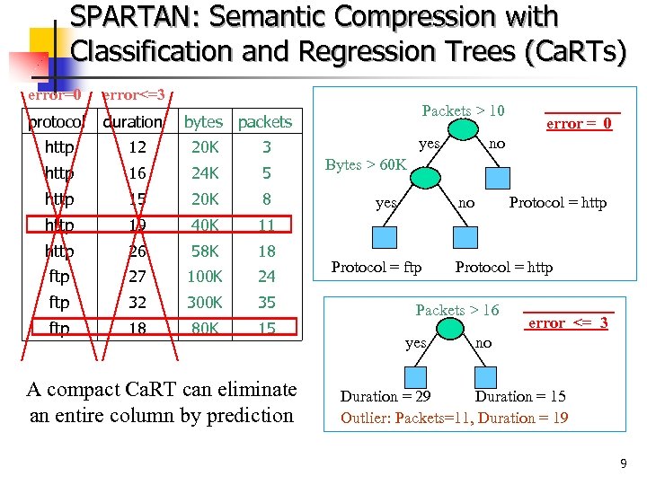SPARTAN: Semantic Compression with Classification and Regression Trees (Ca. RTs) error=0 error<=3 protocol duration http 12 20 K 3 http 16 24 K 5 http 15 20 K 8 http 19 40 K 11 http 26 58 K 18 ftp 27 100 K 24 ftp 32 300 K 35 ftp 18 80 K 15 Packets > 10 bytes packets A compact Ca. RT can eliminate an entire column by prediction yes error = 0 no Bytes > 60 K yes no Protocol = ftp Protocol = http Packets > 16 yes error <= 3 no Duration = 29 Duration = 15 Outlier: Packets=11, Duration = 19 9

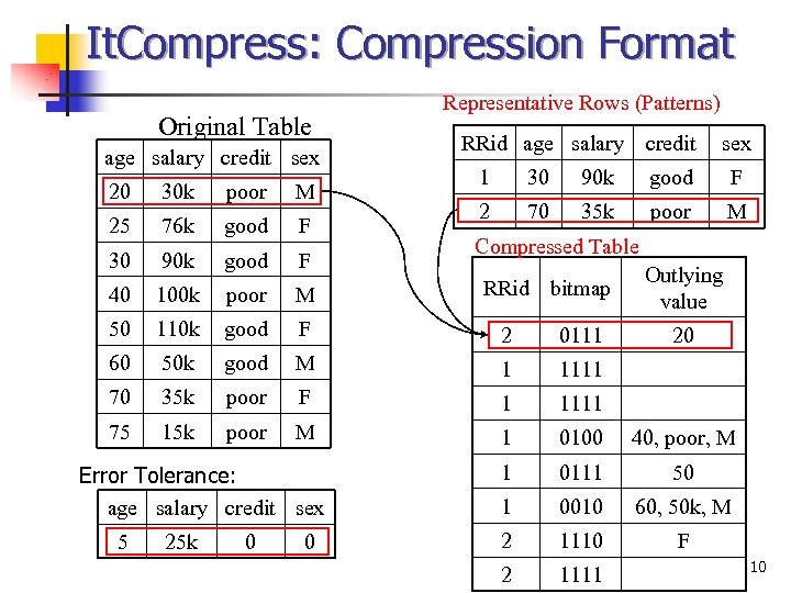It. Compress: Compression Format Original Table age salary credit sex 20 30 k poor M 25 76 k good F 30 90 k good F Representative Rows (Patterns) RRid age salary credit sex 1 30 90 k good F 2 70 35 k poor M Compressed Table RRid bitmap Outlying value 40 100 k poor M 50 110 k good F 2 0111 60 50 k good M 1 1111 70 35 k poor F 1 1111 75 15 k poor M 1 0100 40, poor, M 1 0111 50 1 0010 60, 50 k, M 2 1110 F 2 1111 Error Tolerance: age salary credit sex 5 25 k 0 0 20 10

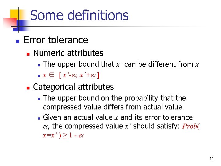Some definitions n Error tolerance n Numeric attributes n n n The upper bound that x’ can be different from x x ∈ [ x’-ei, x’+ei ] Categorical attributes n n The upper bound on the probability that the compressed value differs from actual value Given an actual value x and its error tolerance ei, the compressed value x’ should satisfy: Prob( x=x’ ) ≥ 1 - ei 11

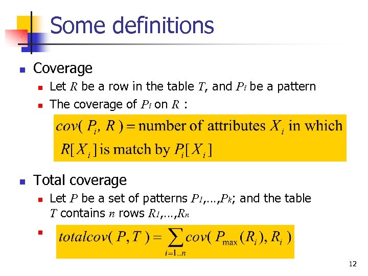Some definitions n Coverage n n n Let R be a row in the table T, and Pi be a pattern The coverage of Pi on R : Total coverage n Let P be a set of patterns P 1, …, Pk; and the table T contains n rows R 1, …, Rn n 12

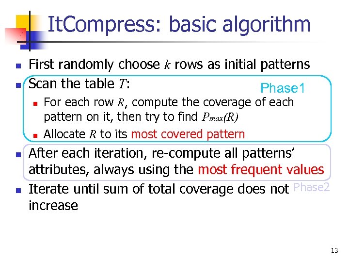It. Compress: basic algorithm n n First randomly choose k rows as initial patterns Scan the table T: Phase 1 n n For each row R, compute the coverage of each pattern on it, then try to find Pmax(R) Allocate R to its most covered pattern After each iteration, re-compute all patterns’ attributes, always using the most frequent values Iterate until sum of total coverage does not Phase 2 increase 13

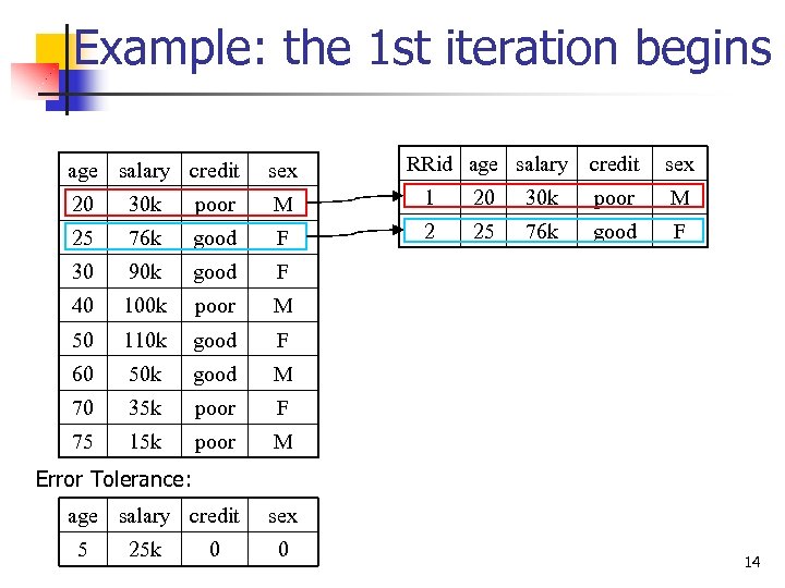Example: the 1 st iteration begins RRid age salary credit sex 20 30 k poor M 1 20 25 76 k good F 2 25 30 90 k good 100 k poor 110 k good 50 k good 35 k poor 15 k poor good F M age salary credit 76 k F 75 M M 70 poor F 60 30 k M 50 sex F 40 credit sex Error Tolerance: 5 25 k 0 0 14

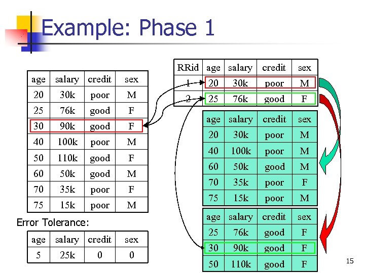Example: Phase 1 RRid age salary credit sex 1 20 30 k poor M 2 25 76 k good F 30 90 k good F 40 100 k poor M 50 110 k good F 60 50 k good M 70 35 k poor F 75 15 k poor M age salary credit 5 25 k 0 sex 20 30 k poor M 40 100 k poor M 60 50 k good M 70 35 k poor F 75 15 k poor M age salary credit Error Tolerance: age salary credit sex 25 76 k good F 30 90 k good F 50 110 k good F 15

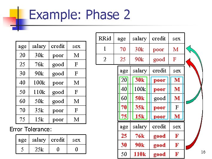Example: Phase 2 RRid age salary credit sex 20 30 k poor M 25 76 k good F 30 90 k good F 40 100 k poor M 50 110 k good F 60 50 k good M 70 35 k poor F 75 15 k poor M age salary credit 25 k salary credit sex 1 20 70 30 k poor M M 2 25 25 90 k 76 k good F F 0 sex 0 age salary credit sex 20 30 k poor M 40 100 k poor M 60 50 k good M 70 35 k poor F 75 15 k poor M age salary credit Error Tolerance: 5 age sex 25 76 k good F 30 90 k good F 50 110 k good F 16

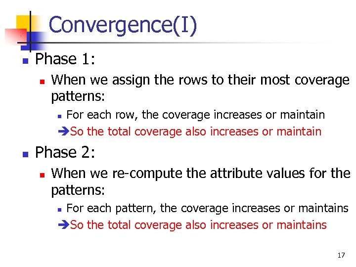Convergence(I) n Phase 1: n When we assign the rows to their most coverage patterns: For each row, the coverage increases or maintain èSo the total coverage also increases or maintain n n Phase 2: n When we re-compute the attribute values for the patterns: For each pattern, the coverage increases or maintains èSo the total coverage also increases or maintains n 17

Convergence(II) n In both Phase 1&2, the total coverage is either increased or maintained, and it has a obvious upper bound (cover the whole table) èThe algorithm will converge eventually 18

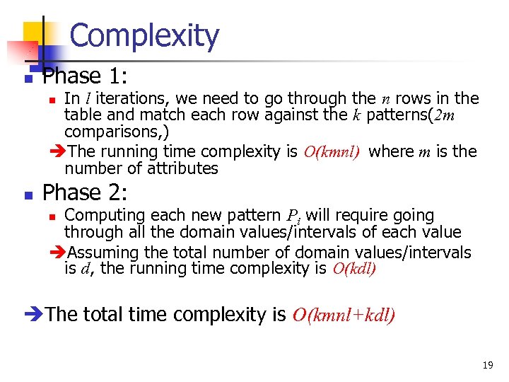Complexity n Phase 1: In l iterations, we need to go through the n rows in the table and match each row against the k patterns(2 m comparisons, ) èThe running time complexity is O(kmnl) where m is the number of attributes n n Phase 2: Computing each new pattern Pi will require going through all the domain values/intervals of each value èAssuming the total number of domain values/intervals is d, the running time complexity is O(kdl) n èThe total time complexity is O(kmnl+kdl) 19

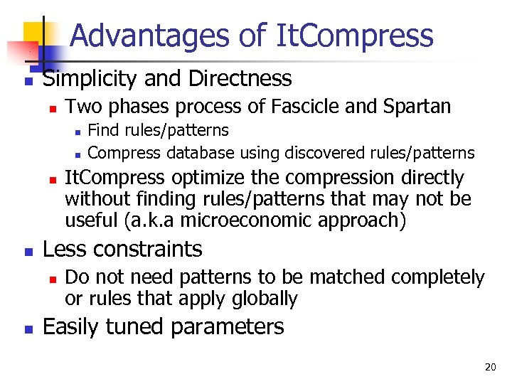Advantages of It. Compress n Simplicity and Directness n Two phases process of Fascicle and Spartan n n It. Compress optimize the compression directly without finding rules/patterns that may not be useful (a. k. a microeconomic approach) Less constraints n n Find rules/patterns Compress database using discovered rules/patterns Do not need patterns to be matched completely or rules that apply globally Easily tuned parameters 20

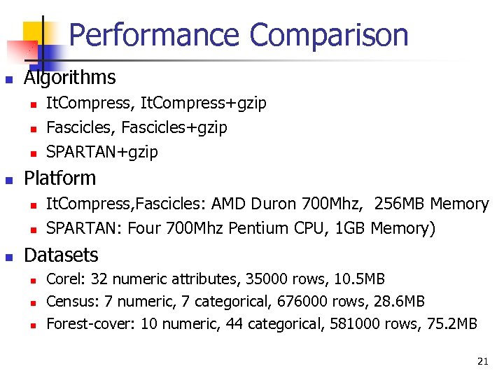Performance Comparison n Algorithms n n Platform n n n It. Compress, It. Compress+gzip Fascicles, Fascicles+gzip SPARTAN+gzip It. Compress, Fascicles: AMD Duron 700 Mhz, 256 MB Memory SPARTAN: Four 700 Mhz Pentium CPU, 1 GB Memory) Datasets n n n Corel: 32 numeric attributes, 35000 rows, 10. 5 MB Census: 7 numeric, 7 categorical, 676000 rows, 28. 6 MB Forest-cover: 10 numeric, 44 categorical, 581000 rows, 75. 2 MB 21

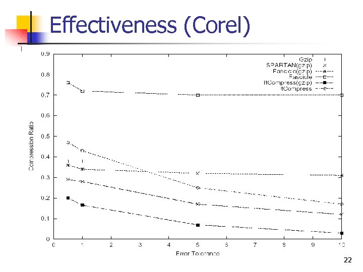Effectiveness (Corel) 22

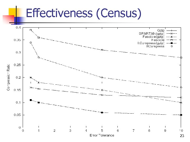Effectiveness (Census) 23

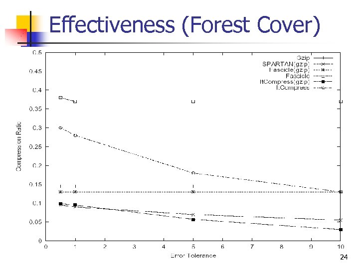Effectiveness (Forest Cover) 24

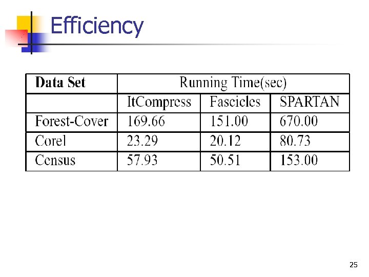Efficiency 25

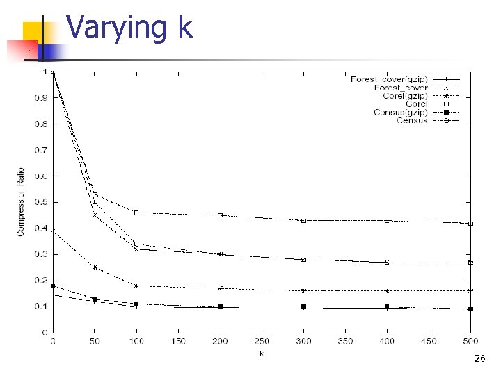Varying k 26

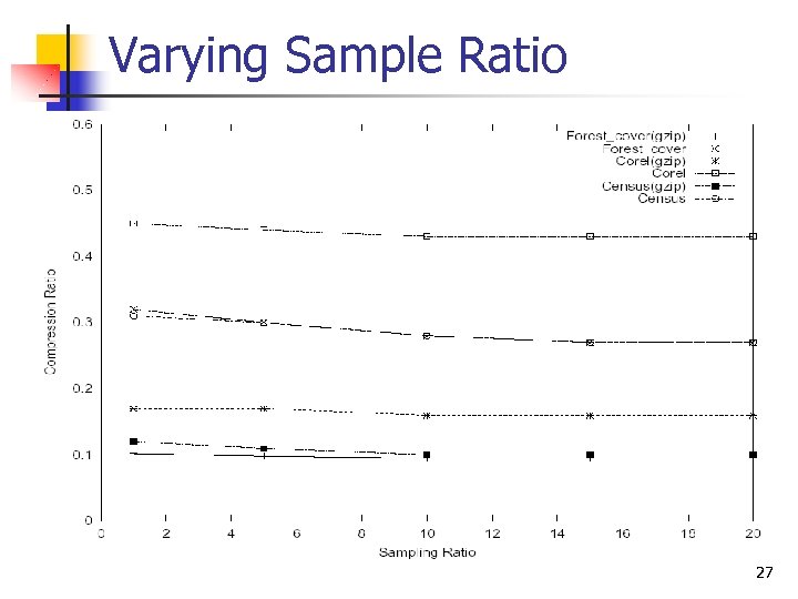Varying Sample Ratio 27

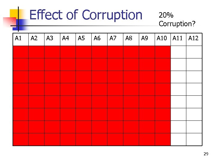
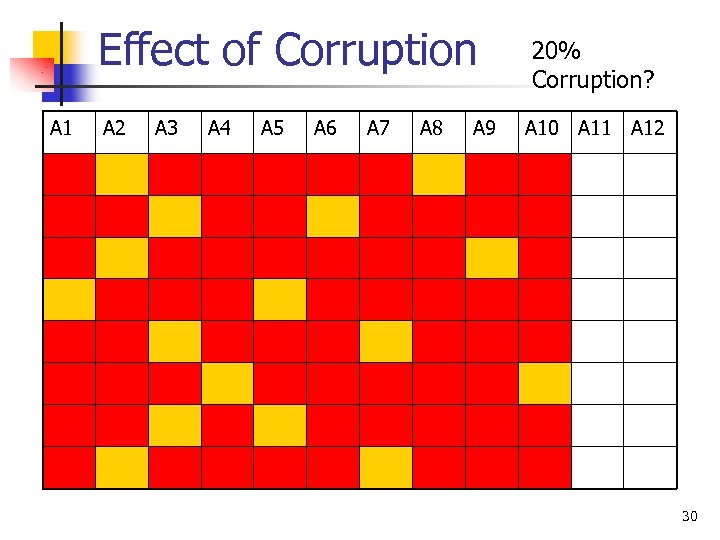
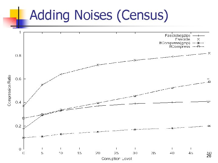Adding Noises (Census) 28

Effect of Corruption A 1 A 2 A 3 A 4 A 5 A 6 A 7 A 8 A 9 20% Corruption? A 10 A 11 A 12 29

Effect of Corruption A 1 A 2 A 3 A 4 A 5 A 6 A 7 A 8 A 9 20% Corruption? A 10 A 11 A 12 30

Findings n It. Compress is n n More efficient than SPARTAN More effective than Fascicles Insensitive to parameter setting Robust to noises 31

Future work n Can we perform mining on the compressed datasets using only the patterns and the bitmap ? n n Example: Building Bayesian Belief Network Is It. Compress a good “bootstrap” semantic compression algorithm ? It. Compress database Other Semantic Compression Algorithms Compressed database 32

Reference List n n S. Babu, M. Garofalakis, and R. Rastogi. SPARTAN: A Model-Based Semantic Compression System for Massive Data Tables. ACM SIGMOD, 2001. H. V. Jagadish, J. Madar, R. T. Ng. Semantic Compression and Pattern Extraction with Fascicles. VLDB, 1999. H. V. Jagadish, R. T. Ng, B. C. Ooi, Anthony K. H. Tung. It. Compress: An Iterative Semantic Compression Algorithm. ICDE 2004. J. Ziv, A. Lempel. A Universal Algorithm for Sequential Data Compression. IEEE Trans, 1977. 33

n Thanks you! 34