Islamic University of Gaza Electrical Engineering Department Communication

Islamic University of Gaza Electrical Engineering Department Communication I laboratory Amplitude modulation DSB-LC (full AM) Submitted by: Adham Abu-Shamla Mohammed Hajjaj 120063320 120063640 Submitted to: Eng. Mohammed kamel Abu-Foul 1

Contents: The objective of this experiment. Quick review about the AM modulation and (DSB-LC) Part 1 code and its comments and results (step by step) Part 2 code and its comment and results Conclusion. 2

Objective: Understanding AM modulation, Double Side Band-Large Carrier (DSB-LC) “known as Full AM”. Using MATLAB to plot the modulated signal. To simulate coherent demodulator and an envelope detector to obtain the real signal using MATLAB. 3

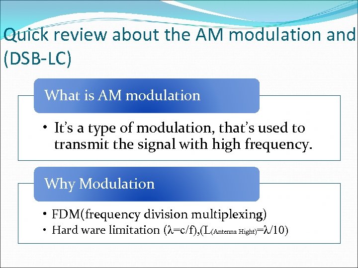Quick review about the AM modulation and (DSB-LC) What is AM modulation • It’s a type of modulation, that’s used to transmit the signal with high frequency. Why Modulation • FDM(frequency division multiplexing) • Hard ware limitation (λ=c/f), (L(Antenna Hight)=λ/10)

Type of AM Modulation 1. 2. 3. 4. DSB-SC DSB-LC SSB VSB

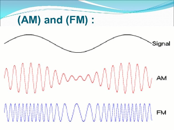(AM) and (FM) : 6

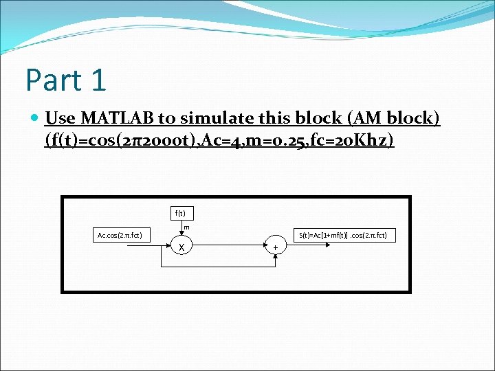Part 1 Use MATLAB to simulate this block (AM block) (f(t)=cos(2π2000 t), Ac=4, m=0. 25, fc=20 Khz) f(t) Ac. cos(2. π. fct) m X S(t)=Ac[1+mf(t)]. cos(2. π. fct) +

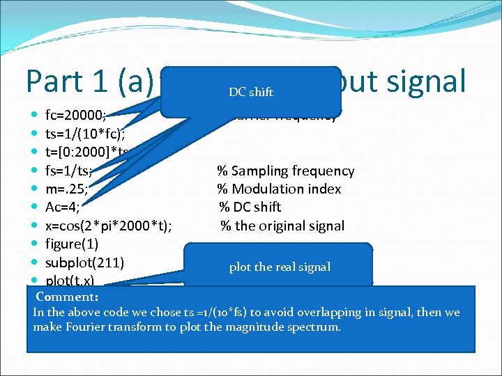Part 1 (a) code: the input signal Modulation index µ=mp/A Carrier shift Sampling period DC frequancy Sampling freqyancy fc=20000; % Carrier frequency ts=1/(10*fc); t=[0: 2000]*ts; fs=1/ts; % Sampling frequency m=. 25; % Modulation index Ac=4; % DC shift x=cos(2*pi*2000*t); % the original signal figure(1) subplot(211) plot the real signal plot(t, x) Comment: of baseband signal x(t)') title('plot In the above code we xlabel('time (t)') chose ts =1/(10*fs) to avoid overlapping in signal, then we make Fourier transform to plot the magnitude spectrum. ylabel('x(t)')

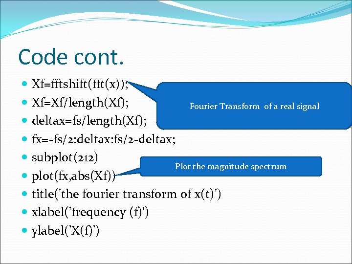Code cont. Xf=fftshift(fft(x)); Xf=Xf/length(Xf); Fourier Transform of a real signal deltax=fs/length(Xf); fx=-fs/2: deltax: fs/2 -deltax; subplot(212) Plot the magnitude spectrum plot(fx, abs(Xf)) title('the fourier transform of x(t)') xlabel('frequency (f)') ylabel('X(f)')

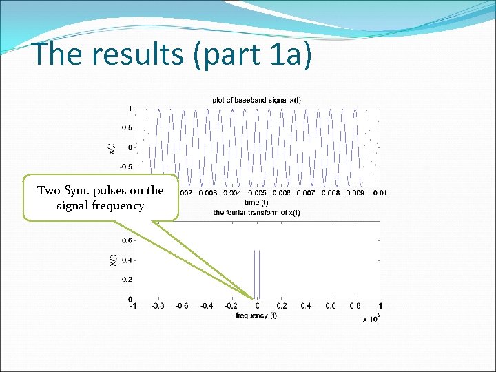The results (part 1 a) Two Sym. pulses on the signal frequency

Code (part 1 b): modulated signal y=(1+m*x)*Ac. *cos(2*pi*fc*t); % (Modulated signal) figure(2) subplot(211) plot(t, y) title('the modulated signal y(t)=(1+m*x)*Ac. *cos(2*pi*fc*t)') xlabel('time (t)') ylabel('y(t)') yf=fftshift(fft(y));

Code (part 1 b): modulated signal cont. yf=yf/length(yf); delta=fs/length(yf); f=-fs/2: delta: fs/2 -delta; subplot(212) Plot the magnitude spectrum plot(f, abs(yf)) title('the fourier transform of the modulated signal Y(f)') xlabel('frequency (f)') ylabel('Y(f)')

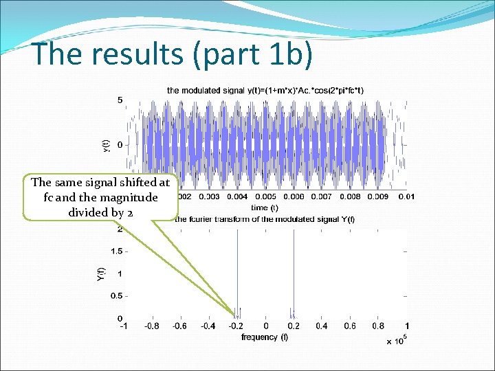The results (part 1 b) The same signal shifted at fc and the magnitude divided by 2

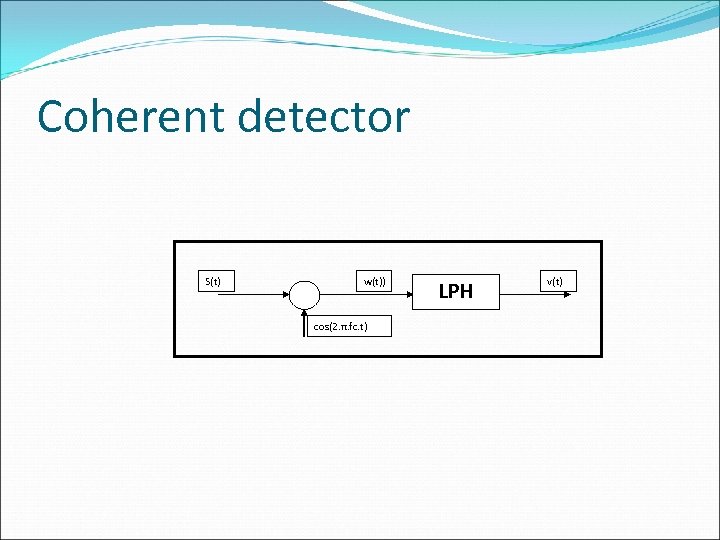Coherent detector S(t) w(t)) cos(2. π. fc. t) LPH v(t)

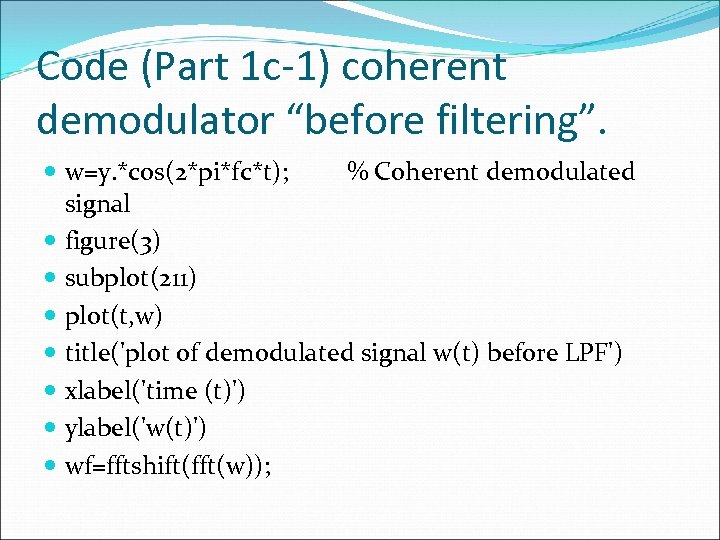Code (Part 1 c-1) coherent demodulator “before filtering”. w=y. *cos(2*pi*fc*t); % Coherent demodulated signal figure(3) subplot(211) plot(t, w) title('plot of demodulated signal w(t) before LPF') xlabel('time (t)') ylabel('w(t)') wf=fftshift(fft(w));

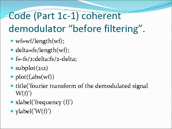Code (Part 1 c-1) coherent demodulator “before filtering”. wf=wf/length(wf); delta=fs/length(wf); f=-fs/2: delta: fs/2 -delta; subplot(212) plot(f, abs(wf)) title('fourier transform of the demodulated signal W(f)') xlabel('frequency (f)') ylabel('W(f)')

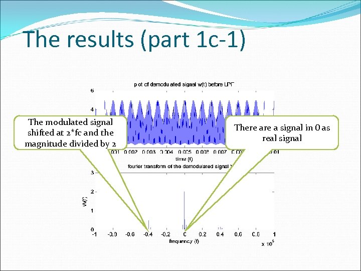The results (part 1 c-1) The modulated signal shifted at 2*fc and the magnitude divided by 2 There a signal in 0 as real signal

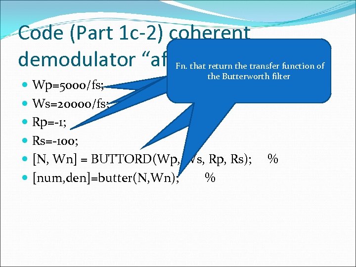Code (Part 1 c-2) coherent demodulator “after filtering”. Fn. that return the transfer function of The Upper frequency of the transient Fn. that return the order of transient the lower frequency of the filter losses due to rippels regionthe Butterworth filterand 1 ) and must be off frequency ( the cutt between 0 Wp=5000/fs; Ws=20000/fs; Rp=-1; Rs=-100; [N, Wn] = BUTTORD(Wp, Ws, Rp, Rs); [num, den]=butter(N, Wn); % %

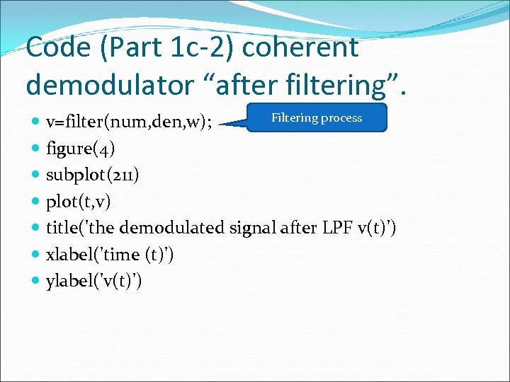Code (Part 1 c-2) coherent demodulator “after filtering”. Filtering process v=filter(num, den, w); figure(4) subplot(211) plot(t, v) title('the demodulated signal after LPF v(t)') xlabel('time (t)') ylabel('v(t)')

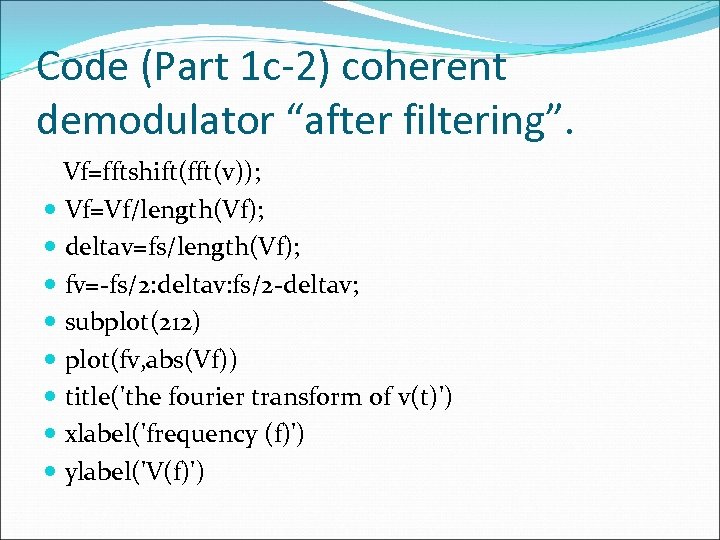Code (Part 1 c-2) coherent demodulator “after filtering”. Vf=fftshift(fft(v)); Vf=Vf/length(Vf); deltav=fs/length(Vf); fv=-fs/2: deltav: fs/2 -deltav; subplot(212) plot(fv, abs(Vf)) title('the fourier transform of v(t)') xlabel('frequency (f)') ylabel('V(f)')

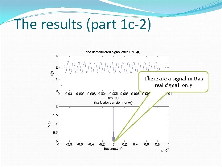The results (part 1 c-2) There a signal in 0 as real signal only

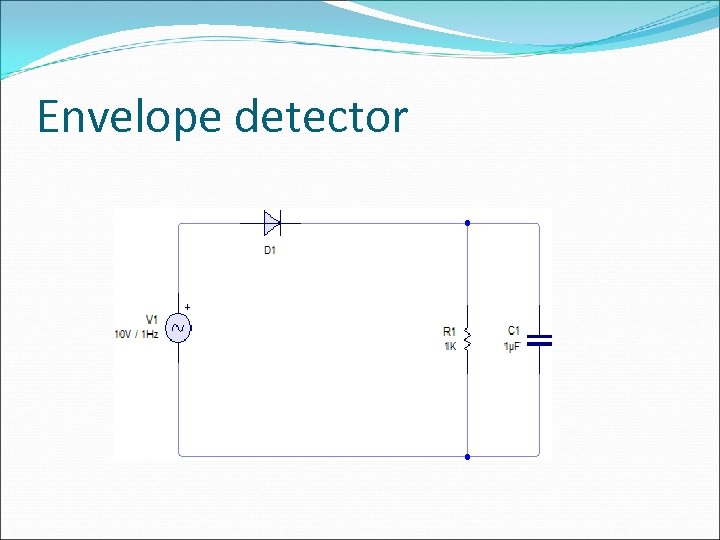Envelope detector

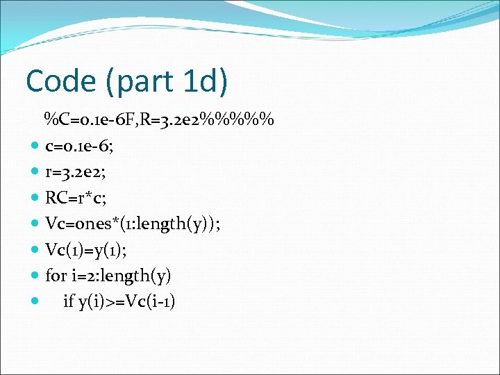Code (part 1 d) %C=0. 1 e-6 F, R=3. 2 e 2%%%%% c=0. 1 e-6; r=3. 2 e 2; RC=r*c; Vc=ones*(1: length(y)); Vc(1)=y(1); for i=2: length(y) if y(i)>=Vc(i-1)

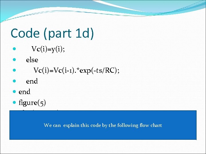Code (part 1 d) Vc(i)=y(i); else Vc(i)=Vc(i-1). *exp(-ts/RC); end figure(5) plot(t, y, t, Vc) %%%%%%%%%%%%%% We can explain this code by the following flow chart %%%%%%%%

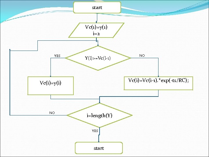start Vc(1)=y(1) i=2 YES Y(i)>=Vc(i-1) Vc(i)=Vc(i-1). *exp(-ts/RC); Vc(i)=y(i) NO NO i=length(Y) YES start

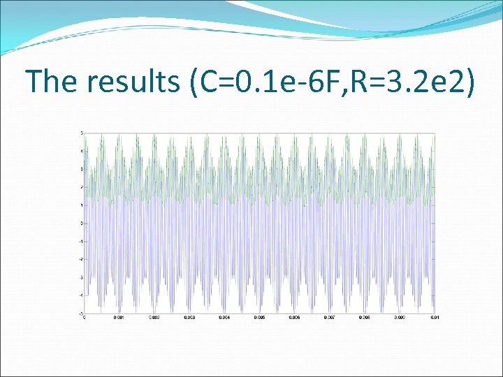The results (C=0. 1 e-6 F, R=3. 2 e 2)

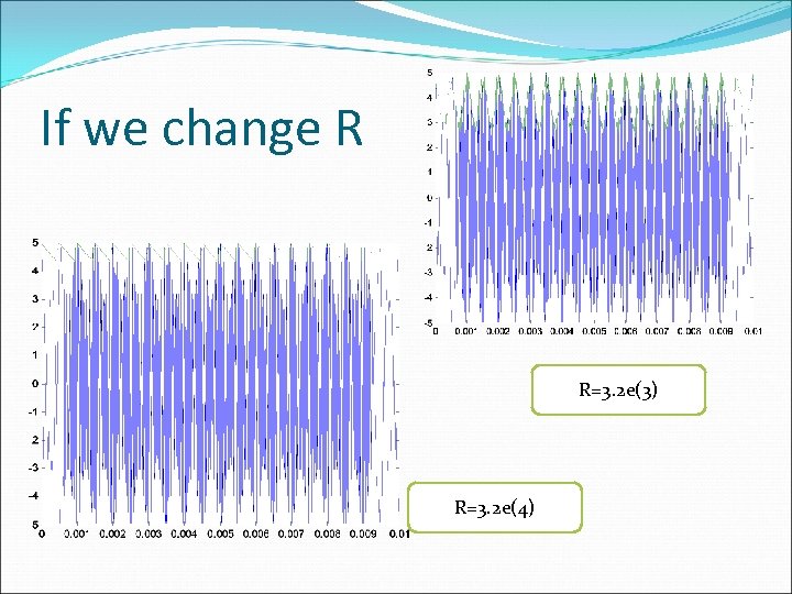If we change R R=3. 2 e(3) R=3. 2 e(4)

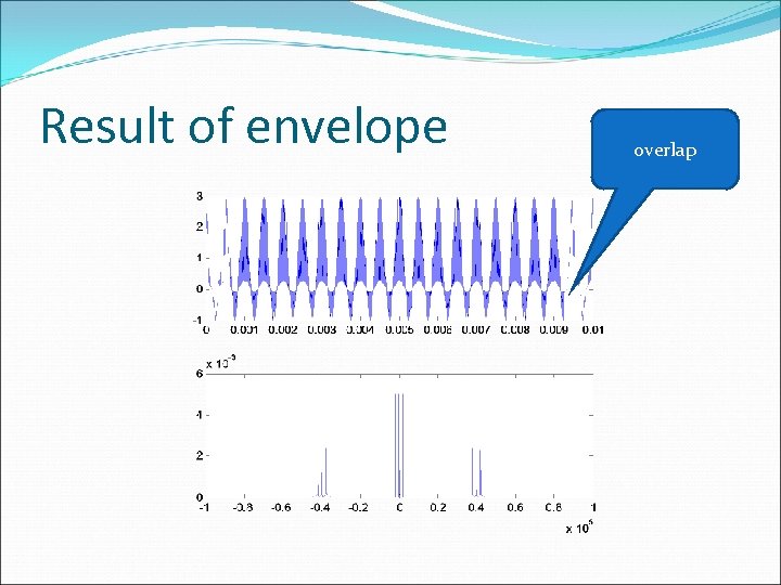
Part 2 Repeat part 1 with Ac=1, m = 2 After we make the simulation, the result is the same in part 1, but we saw some difference in the envelope detector. we will show the results of this part and comment the reason

Result of envelope overlap

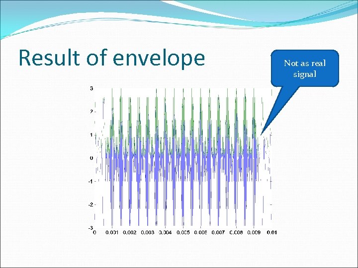Result of envelope Not as real signal

Comment in part 2 The reason of part 2 become like this becouse the Ac is not enough to alternate the signal up to zero so envelope detector can’t get the real signal

Conclusion The experiment is a good simulate for AM signals. We must make sure of the code because any error causes fail in compiling

Thank you