IS MP model consists of IS curve combinations of

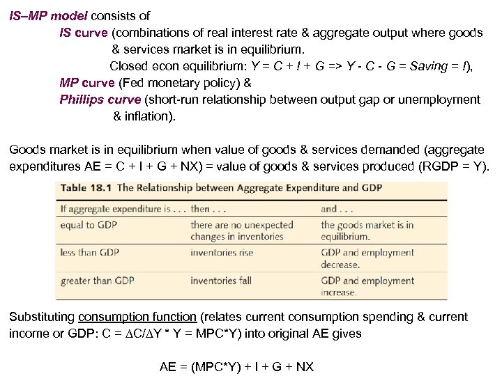
IS–MP model consists of IS curve (combinations of real interest rate & aggregate output where goods & services market is in equilibrium. Closed econ equilibrium: Y = C + I + G => Y - C - G = Saving = I), MP curve (Fed monetary policy) & Phillips curve (short-run relationship between output gap or unemployment & inflation). Goods market is in equilibrium when value of goods & services demanded (aggregate expenditures AE = C + I + G + NX) = value of goods & services produced (RGDP = Y). Substituting consumption function (relates current consumption spending & current income or GDP: C = ∆C/∆Y * Y = MPC*Y) into original AE gives AE = (MPC*Y) + I + G + NX

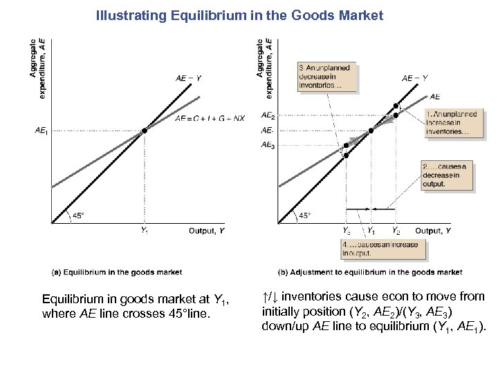
Illustrating Equilibrium in the Goods Market Equilibrium in goods market at Y 1, where AE line crosses 45°line. ↑/↓ inventories cause econ to move from initially position (Y 2, AE 2)/(Y 3, AE 3) down/up AE line to equilibrium (Y 1, AE 1).

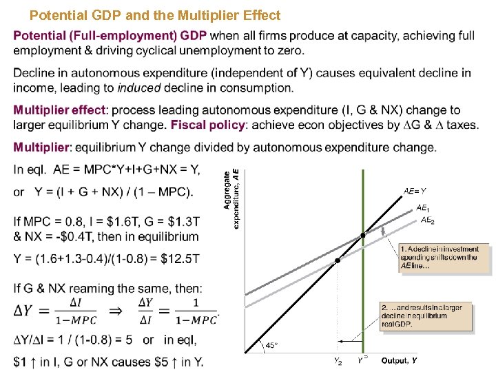
Potential GDP and the Multiplier Effect

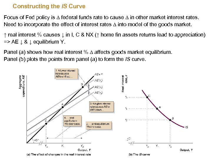
Constructing the IS Curve Focus of Fed policy is ∆ federal funds rate to cause ∆ in other market interest rates. Need to incorporate the effect of interest rates ∆ into model of the goods market. ↑ real interest % causes ↓ in I, C & NX (↑ home fin assets returns lead to appreciation) => AE ↓ & ↓ equilibrium Y. Panel (a) shows how real interest % ∆ affects goods market equilibrium. Panel (b) plots the points from panel (a) to form the IS curve.

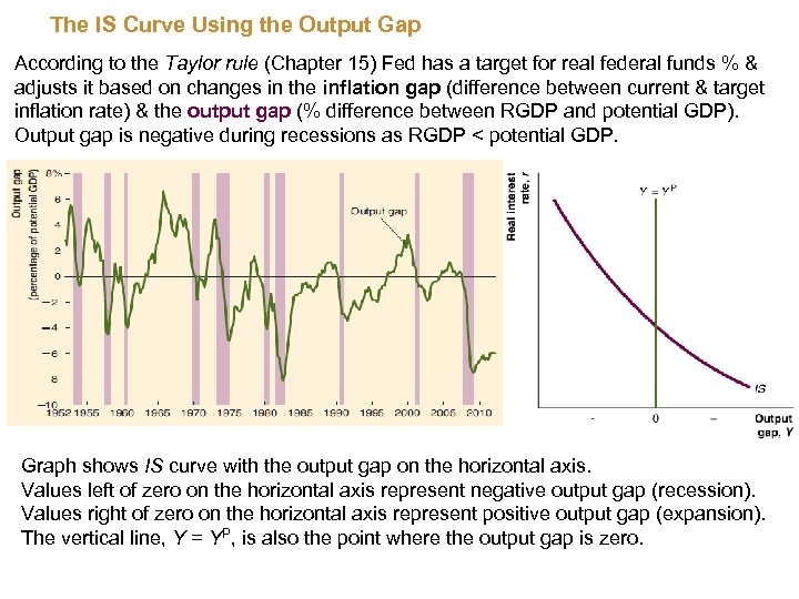
The IS Curve Using the Output Gap According to the Taylor rule (Chapter 15) Fed has a target for real federal funds % & adjusts it based on changes in the inflation gap (difference between current & target inflation rate) & the output gap (% difference between RGDP and potential GDP). Output gap is negative during recessions as RGDP < potential GDP. Graph shows IS curve with the output gap on the horizontal axis. Values left of zero on the horizontal axis represent negative output gap (recession). Values right of zero on the horizontal axis represent positive output gap (expansion). The vertical line, Y = YP, is also the point where the output gap is zero.

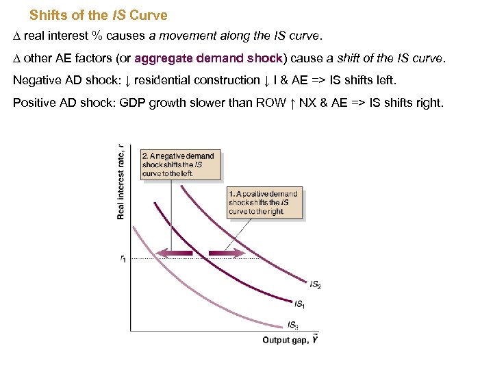
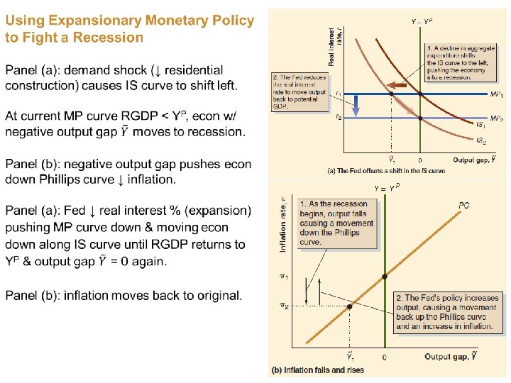
Shifts of the IS Curve ∆ real interest % causes a movement along the IS curve. ∆ other AE factors (or aggregate demand shock) cause a shift of the IS curve. Negative AD shock: ↓ residential construction ↓ I & AE => IS shifts left. Positive AD shock: GDP growth slower than ROW ↑ NX & AE => IS shifts right.

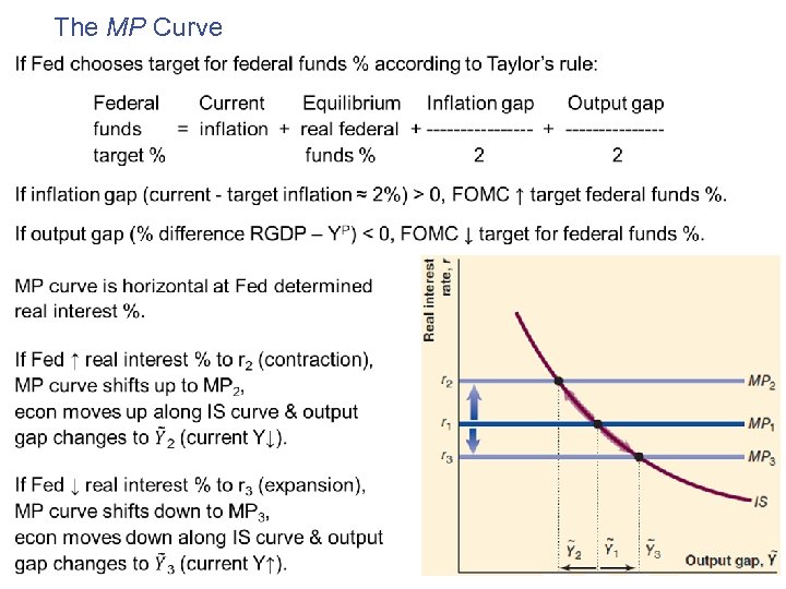
The MP Curve

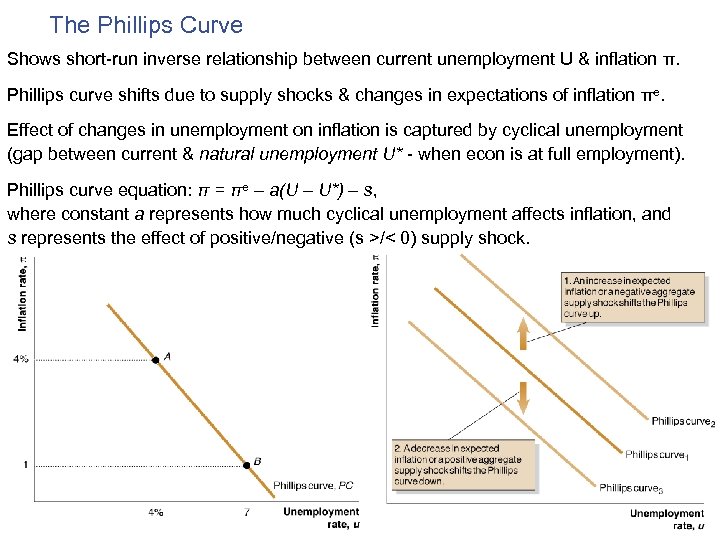
The Phillips Curve Shows short-run inverse relationship between current unemployment U & inflation π. Phillips curve shifts due to supply shocks & changes in expectations of inflation πe. Effect of changes in unemployment on inflation is captured by cyclical unemployment (gap between current & natural unemployment U* - when econ is at full employment). Phillips curve equation: π = πe – a(U – U*) – s, where constant a represents how much cyclical unemployment affects inflation, and s represents the effect of positive/negative (s >/< 0) supply shock.

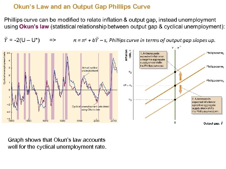
Okun’s Law and an Output Gap Phillips Curve Graph shows that Okun’s law accounts well for the cyclical unemployment rate.

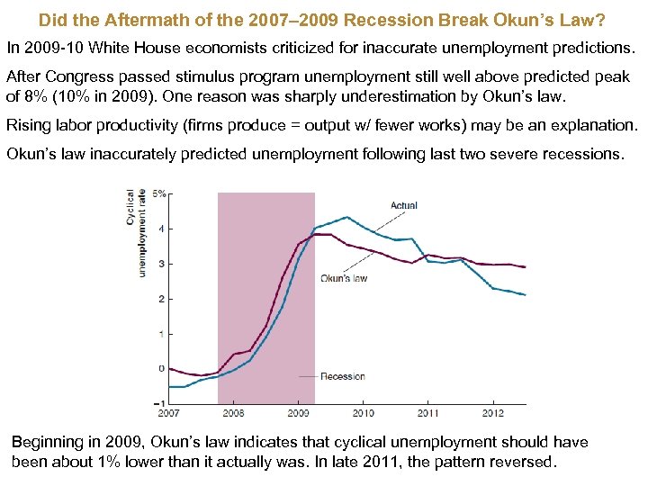
Did the Aftermath of the 2007– 2009 Recession Break Okun’s Law? In 2009 -10 White House economists criticized for inaccurate unemployment predictions. After Congress passed stimulus program unemployment still well above predicted peak of 8% (10% in 2009). One reason was sharply underestimation by Okun’s law. Rising labor productivity (firms produce = output w/ fewer works) may be an explanation. Okun’s law inaccurately predicted unemployment following last two severe recessions. Beginning in 2009, Okun’s law indicates that cyclical unemployment should have been about 1% lower than it actually was. In late 2011, the pattern reversed.

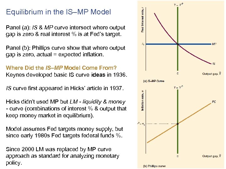
Equilibrium in the IS–MP Model Panel (a): IS & MP curve intersect where output gap is zero & real interest % is at Fed’s target. Panel (b): Phillips curve show that where output gap is zero, actual = expected inflation. Where Did the IS–MP Model Come From? Keynes developed basic IS curve ideas in 1936. IS curve first appeared in Hicks’ article in 1937. Hicks didn’t used MP but LM - liquidity & money - curve (combinations of interest % & output that keep money market in equilibrium). Model assumes Fed targets money supply, but since early 1980 s Fed targets federal funds %. Since 2000 LM was replaced by MP curve approach as standard for analyzing monetary policy.

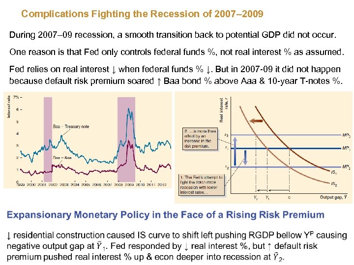
Complications Fighting the Recession of 2007– 2009 During 2007– 09 recession, a smooth transition back to potential GDP did not occur. One reason is that Fed only controls federal funds %, not real interest % as assumed. Fed relies on real interest ↓ when federal funds % ↓. But in 2007 -09 it did not happen because default risk premium soared ↑ Baa bond % above Aaa & 10 -year T-notes %.

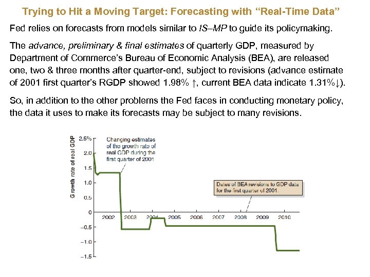
Trying to Hit a Moving Target: Forecasting with “Real-Time Data” Fed relies on forecasts from models similar to IS–MP to guide its policymaking. The advance, preliminary & final estimates of quarterly GDP, measured by Department of Commerce’s Bureau of Economic Analysis (BEA), are released one, two & three months after quarter-end, subject to revisions (advance estimate of 2001 first quarter’s RGDP showed 1. 98% ↑, current BEA data indicate 1. 31%↓). So, in addition to the other problems the Fed faces in conducting monetary policy, the data it uses to make its forecasts may be subject to many revisions.

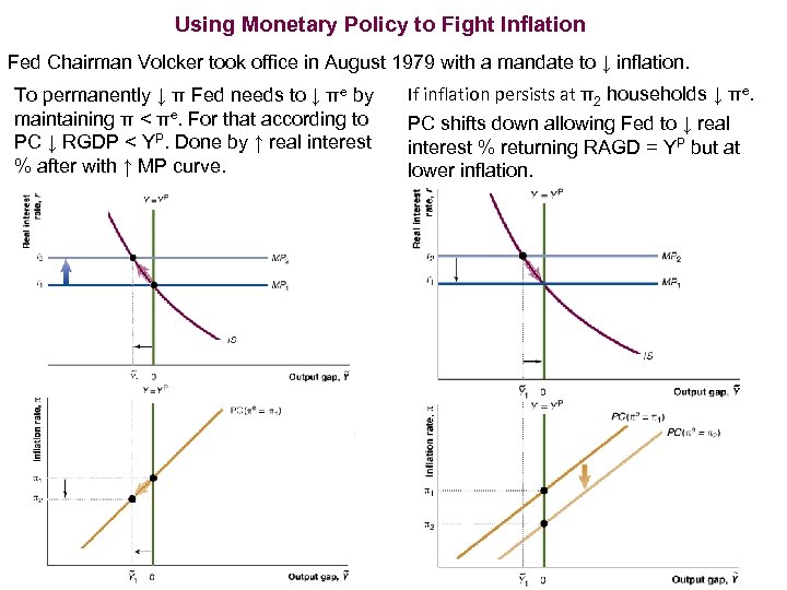
Using Monetary Policy to Fight Inflation Fed Chairman Volcker took office in August 1979 with a mandate to ↓ inflation. To permanently ↓ π Fed needs to ↓ πe by maintaining π < πe. For that according to PC ↓ RGDP < YP. Done by ↑ real interest % after with ↑ MP curve. If inflation persists at π2 households ↓ πe. PC shifts down allowing Fed to ↓ real interest % returning RAGD = YP but at lower inflation.

Monetary Policy Channels Ways in which monetary policy affects output & prices. In IS-MP model monetary policy works through interest rate channel: Fed uses open market operations to ∆ real interest %, to ∆ AE, to ∆ output gap & inflation. Key assumption: borrowers indifferent to how or from whom they raise funds & alternative sources of funds are close substitutes. Bank lending channel how monetary policy influences spending by borrowers. Monetary expansion (↓ %) causes ↑ AE for ↑ loan availability & ↑ borrowers’ spending. If banks ↑ deposits by ↓ loan %, what borrowers can borrow & spend ↑ at any real %. So, monetary expansion effectiveness is independent of interest rates reduction. ↑ Y occurs because lower federal funds % causes other interest % to fall. Both channels similar in one respect: ↑ bank reserves leads to ↓ loan interest % which through competition ↓ interest % in financial markets. Balance sheet channel how interest rate ∆ resulting from monetary policy affect borrowers’net worth (= TA – TL), liquidity & spending. Even if monetary policy doesn’t affect banks’ ability to lend, monetary expansion ↑ borrowers’net worth ↑ AD & ↑ Y.

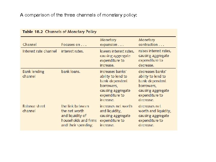
A comparison of the three channels of monetary policy: