

73b307c6c783be75937e48245a32b6e9.ppt
- Количество слайдов: 68
 Ionosphere and Neutral Atmosphere • Temperature and density structure • Hydrogen escape • Thermospheric variations and satellite drag • Mean wind structure
; “change” Lots of weather Strato (Latin: stratum); Layered Meso (Greek: messos);") Tropo (Greek: tropos); “change” Lots of weather Strato (Latin: stratum); Layered Meso (Greek: messos); Middle Thermo (Greek: thermes); Heat Exo (greek: exo); outside
Tropo (Greek: tropos); “change” Lots of weather Strato (Latin: stratum); Layered Meso (Greek: messos); Middle Thermo (Greek: thermes); Heat Exo (greek: exo); outside
.") Variation of the density in an atmosphere with constant temperature (750 K).
Variation of the density in an atmosphere with constant temperature (750 K).
 • Composition of the dayside ionosphere under solar minimum conditions. – At low altitudes the major ions are O 2+ and NO+ – Near the F 2 peak it changes to O+ – The topside ionosphere becomes H+ dominant. • • • For practical purposes the ionosphere can be thought of as quasi-neutral (the net charge is practically zero in each volume element with enough particles). The ionosphere is formed by ionization of the three main atmospheric constituents N 2, O 2, and O. The primary ionization mechanism is photoionization by extreme ultraviolet (EUV) and X-ray radiation. – In some areas ionization by particle precipitation is also important. • The ionization process is followed by a series of chemical reactions – Recombination removes free charges and transforms the ions to neutral particles.
 • Neutral density exceeds the ion density below about 500 km.
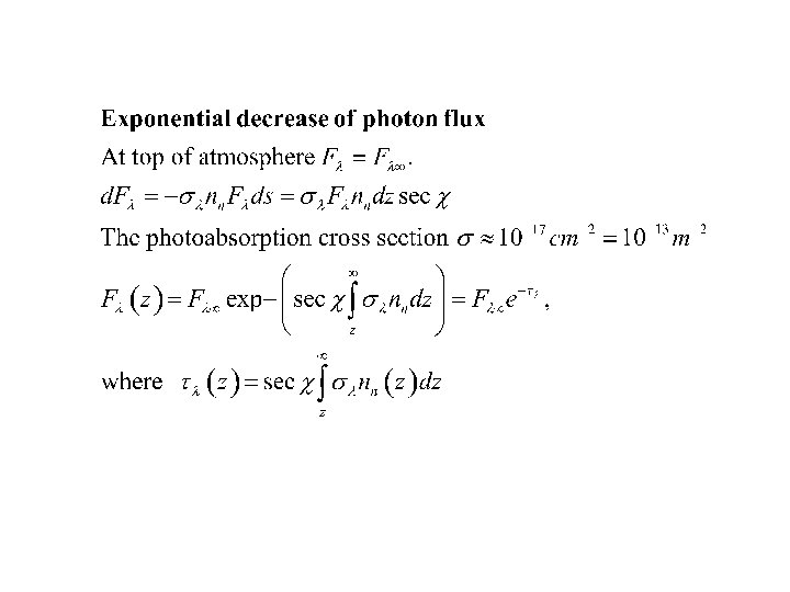
 • Let the photon flux per unit frequency be – The change in the flux due to absorption by the neutral gas in a distance ds is where n(z) is the neutral gas concentration, is the frequency dependent photo absorption cross section, and ds is the path length element in the direction of the optical radiation. (Assuming there are no other local sources or sinks of ionizing radiation. ) – (where is the zenith angle of the incoming solar radiation. – The altitude dependence of the solar radiation flux becomes where is the incident photon intensity per unit frequency. – is called the optical depth. – There is usually more than one atmospheric constituent attenuating the photons each of which has its own cross section.
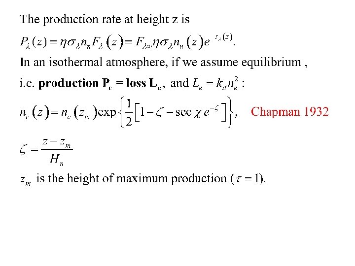
 of the neutral upper atmosphere usually obeys") • • • The density (ns) of the neutral upper atmosphere usually obeys a hydrostatic equation where m is the molecular or atomic mass, g is the acceleration due to gravity, z is the altitude and p=nk. T is thermal pressure. If the temperature T is assumed independent of z, this equation has the exponential solution where is the scale height of the gas, and n 0 is the density at the reference altitude z 0. For this case • For multiple species • The optical depth increases exponentially with decreasing altitude. In thermosphere solar radiation is absorbed mainly via ionization processes. Let us assume that Each absorbed photon creates a new electron-ion pair therefore the electron production is • • where Si is the total electron production rate (particles cm-3 s-1).
• • • The density (ns) of the neutral upper atmosphere usually obeys a hydrostatic equation where m is the molecular or atomic mass, g is the acceleration due to gravity, z is the altitude and p=nk. T is thermal pressure. If the temperature T is assumed independent of z, this equation has the exponential solution where is the scale height of the gas, and n 0 is the density at the reference altitude z 0. For this case • For multiple species • The optical depth increases exponentially with decreasing altitude. In thermosphere solar radiation is absorbed mainly via ionization processes. Let us assume that Each absorbed photon creates a new electron-ion pair therefore the electron production is • • where Si is the total electron production rate (particles cm-3 s-1).
 • Substituting for n and gives where • • The maximum rate of ionization is given by • • This is the Chapman ionization function. If we further assume that the main loss process is ion-electron recombination with a coefficient The altitude of maximum ionization can be obtained by looking for extremes in this equation by calculating • This gives • Choose z 0 as the altitude of maximum ionization for perpendicular solar radiation • This gives and assume that the recombination rate is • Finally if we assume local equilibrium between production and loss we get
 • The vertical profile in a simple Chapman layer is • The E and F 1 regions are essentially Chapman layers while additional production, transport and loss processes are necessary to understand the D and F 2 regions.
 O N
O N
.") Variation of the density in an atmosphere with constant temperature (750 K).
Variation of the density in an atmosphere with constant temperature (750 K).
 • The ionosphere vertical density pattern shows a strong diurnal variation and a solar cycle variation. • Identification of ionospheric layers is related to inflection points in the vertical density profile. Primary Ionospheric Regions Region Altitude Density D 60 -90 km 80 km ~108 – 1010 m-3 E 90 -140 km 110 km ~1011 m-3 F 1 140 -200 km ~1011 -1012 m-3 F 2 below peak Bottom side Peak 200 -400 km ~1012 m-3 Topside F 2 above peak 400 -1000 km ~108 – 1012 m-3
 • Diurnal and solar cycle variation in the ionospheric density profile. – In general densities are larger during solar maximum than during solar minimum. – The D and F 1 regions disappear at night. – The E and F 2 regions become much weaker. – The topside ionosphere is basically an extension of the magnetosphere.
 • The D Region – The most complex and least understood layer in the ionosphere. – The primary source of ionization in the D region is ionization by solar X-rays and Lymanionization of the NO molecule. – Precipitating magnetospheric electrons may also be important. – The primary positive ions are O 2+ and NO+ – The most common negative ion is NO 3 -
 • The E Region – Essentially a Chapman layer formed by Extreme UV ionization. – The main ions are O 2+ and NO+ – Although nitrogen (N 2) molecules are the most common in the atmosphere N 2+ is not common because it is unstable to charge exchange. For example – Oxygen ions are removed by the following reactions
 • The F 1 Region – Essentially a Chapman layer. – The ionizing radiation is EUV at <91 nm. – It is basically absorbed in this region and does not penetrate into the E region. – The principal initial ion is O+. – O+ recombines in a two step process. • First atom ion interchange takes place • This is followed by dissociative recombination of O 2+ and NO+
 • The F 2 Region – The major ion is O+. – This region cannot be a Chapman layer since the atmosphere is optically thin to most ionizing radiation. – This region is formed by an interplay between ion sources and sinks. – The dominant ionization source is photoionization of atomic oxygen – O+ are lost by a two step process • First atom-ion interchange • Dissociative recombination – The peak forms because the loss rate falls off more rapidly than the production rate. – The density falls off at higher altitudes because of diffusion- no longer in local photochemical equilibrium.
 At 80 -100 km, the time constant for mixing is more efficient than recombination, so mixing due to turbulence and other dynamical processes must be taken into account (i. e. , photochemical equilibrium does not hold). Mixing transports O down to lower (denser) levels where recombination proceeds rapidly (the "sink" for O). O Concentration After the O recombines to produce O 2, the O 2 is transported upward by turbulent diffusion to be photodissociated once again (the "source" for O).
 of the ionosphere • in situ – rockets, low-orbital satellites • remote") Sensing (probing) of the ionosphere • in situ – rockets, low-orbital satellites • remote radio sounding (reflection scattering) – ionosondes, coherent/incoherent radars. • remote radio occultation – satellite-ground/ satellites-satellites propagation. • remote optic – sensing natural frequencies of atoms or molecules emission.
Sensing (probing) of the ionosphere • in situ – rockets, low-orbital satellites • remote radio sounding (reflection scattering) – ionosondes, coherent/incoherent radars. • remote radio occultation – satellite-ground/ satellites-satellites propagation. • remote optic – sensing natural frequencies of atoms or molecules emission.
 Radio Sounding • What is radio sounding – Remote sensing with radio waves • Earth space physics applications – Ionosphere – Magnetosphere 20
 DPS 4 RC VA RR AY RCV ANTENNA • small-medium size instruments • low power: 100 s Watts • operating frequency: 1 -20 MHz • target of radar: 2 D surfaces of constant electron density • measures electron density profile, drift velocities • utilized physics phenomenon: resonance at plasma frequency XMT ANTENNA Ionosondes
 Principles of ionosondes • using multiple frequencies to sense plasma at different heights • ionosonde measures delay between transmission and receiving at each freq. • based on this information we can compute electron density profile
 Ionogram and Plasma Density Inversion Electron density profile 23
 at the Magnetic Equator Cachimbo 16 October 2002 noon midnight 24") Ne(h, t) at the Magnetic Equator Cachimbo 16 October 2002 noon midnight 24
Ne(h, t) at the Magnetic Equator Cachimbo 16 October 2002 noon midnight 24
 Ionosonde Field of View and ISR Radar Pencil Beam Specular Reflection and Scatter Radio Sounding: specular reflection wide beam Scatter Radar: Scatter, pencil beam Ionosonde
 Radio Sounding Principles • Waves in a plasma experience reflection and refraction • Radio waves are reflected at wave cutoffs (n = 0) • Echoes are received if the gradient at the reflection point is normal to the incident signals. • The echo frequency gives the plasma conditions of the reflection point, and the time delay gives the distance of reflection point. • From a series of sounding frequencies, a density profile can be obtained n>0 n=0 n<0 Refracted rays Echo Reflected ray Refracted rays SOUNDER
 Ionospheric Drift Measurements • Fourier analysis for Doppler spectra • Interferometry with spaced receive antennas
 Interferometric Doppler Imaging The digisonde, operating in the skymap/drift mode, is designed to measure the drift velocity components on a routine basis. In this mode the ionosonde sounds at one or more fixed frequencies and receives and records the reflected signal from each antenna separately. This technique depends on the presence of ionospheric structures that are embedded in the background plasma. 28
 Digisonde Skymaps: Reflections and Doppler Shifts 29
 Coherent radars • big instruments • very high power: 10 k. Watts • operating frequency: 10 -20 MHz • target of radar: 1 D field aligned structures • measures density and velocity of the target • utilized physics phenomenon: resonance at plasma frequency
 Virginia Tech Super. DARN HF Radars Kapuskasing, Ontario, Canada Goose Bay, Newfoundland Labrador, Canada Fort Hays, Kansas, USA Blackstone, Virginia, USA
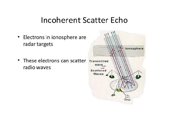
 Incoherent scattering radars • very big instruments • very high power: 1 -10 MWatts • operating frequency: 100 s MHz • no generic design, most common design is steerable/nonsteerable dishes • target of radar: individual electrons/ions • measures density, bulk velocity of the plasma (winds), electron/ion temperature. • utilized physics phenomenon: interaction of charge particle with EM wave Millstone Hill radar
 GNNS total electron content • satellite-ground based receiver technique • detection of a change in a radio signal (phase difference between two operating bands) as it passes through the ionosphere. • the magnitude of the phase shift depends on electron density along the path and is proportional to total electron content • utilized physic phenomenon: Faraday rotation
 • satellite-satellite technique • detection of a change in a radio") Radio occultation (tomography) • satellite-satellite technique • detection of a change in a radio signal (refraction) as it passes through the planet's atmosphere/ionosphere. • the magnitude of the refraction depends on ionosphere / neutral atmosphere density along the path. • for ionosphere radio occultation gives the total electron content • in the case of the neutral atmosphere (below the ionosphere) information on the atmosphere's temperature, pressure and water vapor content can be derived. • when there are enough measurements it is possible to invoke tomography algorithms and derive electron density profile • utilized physics phenomenon: refraction of radio waves
Radio occultation (tomography) • satellite-satellite technique • detection of a change in a radio signal (refraction) as it passes through the planet's atmosphere/ionosphere. • the magnitude of the refraction depends on ionosphere / neutral atmosphere density along the path. • for ionosphere radio occultation gives the total electron content • in the case of the neutral atmosphere (below the ionosphere) information on the atmosphere's temperature, pressure and water vapor content can be derived. • when there are enough measurements it is possible to invoke tomography algorithms and derive electron density profile • utilized physics phenomenon: refraction of radio waves
 • as") Optical methods • detection of the natural frequencies of emission (mainly oxygen) • as well as TEC measurements these methods can only give content along the path • measurement of particular ion concentration not total plasma concentration. • utilized physical phenomenon: individul emission wave length Limb sensing All sky imager (pseudo color)
Optical methods • detection of the natural frequencies of emission (mainly oxygen) • as well as TEC measurements these methods can only give content along the path • measurement of particular ion concentration not total plasma concentration. • utilized physical phenomenon: individul emission wave length Limb sensing All sky imager (pseudo color)
 O N
O N
 Real Time Digisonde F-Region Drift Measurements 39
 IMAGE Spacecraft 20 -m dipole along z 500 -m dipoles in spin plane Launched 25 Mar 2000 RPI: <10 W radiated power 3 k. Hz – 3 MHz 300 Hz bandwidth 40
 RPI IMAGE Instrument Deck 41
 RPI on IMAGE Electronics Unit 42
 43 Sounding in Magnetosphere
 Field-Aligned Propagation RPI Plasmagram Fig 2 of GRL paper 44 (Reinisch et al. , GRL, 2002)
 Plasma Density Along Field line 45
 One Pass of IMAGE on June 8, 2001 IMAGE trajectory 46
 Two dimensional density distribution for MLT=8. 0 on June 8, 2001 47
 Plasmasphere Depleting and Refilling Storm DST full depleted Lppstorm full 48
 Before Storm Partial Recovery Storm Peak • Identified plasmasphere, plasma trough, density depletion, aurora/cusp, and polar cap • The densities and the locations of these regions vary in accordance with the different solar wind/IMF conditions, not correlated with the Dst variations 49
 Before Storm Partial Recovery Storm Peak • Acceleration regions 50
 Ionospheric Topside Sounding TOPAS TOPside Automated Sounder Ionosphere Disturbance Tx TOPAS Vertical Echo Disturbance 51
 TOPAS : Topside Plasma Radar 52
 Dual-Frequency Precision Ranging Swarm spacecraft configuration for precision interferometry -- 0. 1 W transmissions from each s/c -- Each s/c transmits own frequency -- Each s/c receives all frequencies Swarm performs as a multi-antenna interferometer for precision angle-of-arrival measurements --High resolution interferometry for detection of radio transmitters 53
 Magnetospheric Tomography • A 7 -satellite constellation • Each satellite transmits and receives signals • Tomography methods are used to infer the plasma density distribution within the constellation 54
 Digisonde Network
") • The dense regions of the ionosphere (the D, E and F regions) contain concentrations of free electrons and ions. These mobile charges make the ionosphere highly conducting. • Electrical currents can be generated in the ionosphere. • The ionosphere is collisional. Assume that it has an electric field but for now no magnetic field. The ion and electron equations of motion will be where is the ion neutral collision frequency and neutral collision frequency. is the electron – For this simple case the current will be related to electric field by where is a scalar conductivity. • If there is a magnetic field there are magnetic field terms in the momentum equation. In a coordinate system with along the z-axis the conductivity becomes a tensor.
• The dense regions of the ionosphere (the D, E and F regions) contain concentrations of free electrons and ions. These mobile charges make the ionosphere highly conducting. • Electrical currents can be generated in the ionosphere. • The ionosphere is collisional. Assume that it has an electric field but for now no magnetic field. The ion and electron equations of motion will be where is the ion neutral collision frequency and neutral collision frequency. is the electron – For this simple case the current will be related to electric field by where is a scalar conductivity. • If there is a magnetic field there are magnetic field terms in the momentum equation. In a coordinate system with along the z-axis the conductivity becomes a tensor.
 • Specific conductivity – along the magnetic field • Pedersen conductivity – in the direction of the applied electric field • Hall conductivity – in the direction perpendicular to the applied field where and are the total electron and ion momentum transfer collision frequencies and are the electron and ion gyrofrequencies. • The Hall conductivity is important only in the D and E regions. • The specific conductivity is very important for magnetosphere and ionosphere physics. If all field lines would be equipotentials. • The total current density in the ionosphere is
 plasmas undergo") • Within the high latitude magnetosphere (auroral zone and polar cap) plasmas undergo a circulation cycle. – At the highest latitudes the geomagnetic field lines are “open” in that only one end is connected to the Earth. – Ionospheric plasma expands freely in the flux tube as if the outer boundary condition was zero pressure. • For H+ and He+ plasma enters the flux tube at a rate limited by the source. • The net result is a flux of low density supersonic cold light ions into the lobes. • The surprising part is that comparable O+ fluxes also are observed.
• Within the high latitude magnetosphere (auroral zone and polar cap) plasmas undergo a circulation cycle. – At the highest latitudes the geomagnetic field lines are “open” in that only one end is connected to the Earth. – Ionospheric plasma expands freely in the flux tube as if the outer boundary condition was zero pressure. • For H+ and He+ plasma enters the flux tube at a rate limited by the source. • The net result is a flux of low density supersonic cold light ions into the lobes. • The surprising part is that comparable O+ fluxes also are observed.
 Vertical distribution of density and temperature for high solar activity (F 10. 7 = 250) at noon (1) and midnight (2), and for low solar activity (F 10. 7 = 75) at noon (3) and midnight (4) according to the COSPAR International Reference Atmosphere (CIRA) 1965.
 Atmospheric Compositions Compared The atmospheres of Earth, Venus and Mars contain many of the same gases, but in very different absolute and relative abundances. Some values are lower limits only, reflecting the past escape of gas to space and other factors.
 Average Temperature Profiles for Earth, Mars & Venus Mars Venus night day Venus Earth
 Formation of Ionospheres
 HYDROSTATIC EQUILIBRIUM If …. . n = # molecules per unit volume P + d. P m = mass of each particle nm dh = total mass contained in a cylinder of air (of unit cross-sectional area) Then, the force due to gravity on the cylindrical mass = g nmdh and the difference in pressure between the lower and upper faces of the cylinder balances the above force in an equilibrium situation: d. P nmgdh P
 Assuming the ideal gas law holds, Then the previous expression may be written: where H is called the scale height and
 This is the so-called hydrostatic law or barometric law. Integrating, where and z is referred to as the "reduced height" and the subscript zero refers to a reference height at h=0. Similarly, For an isothermal atmosphere, then,
 Absorption of Solar Radiation vs. Height and Species