Inventory Management 12 Power Point presentation to accompany

Inventory Management 12 Power. Point presentation to accompany Heizer and Render Operations Management, Eleventh Edition Principles of Operations Management, Ninth Edition Power. Point slides by Jeff Heyl © 2014 Pearson Education, Inc. © 2014 Pearson Education, 12 - 1

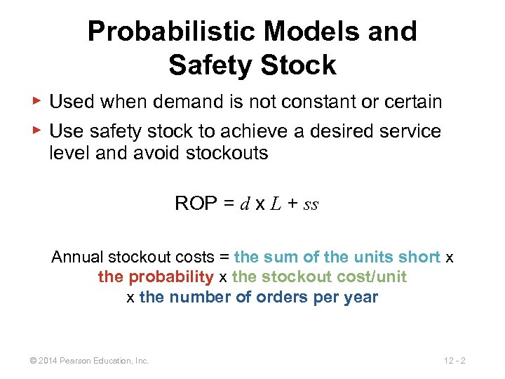Probabilistic Models and Safety Stock ▶ Used when demand is not constant or certain ▶ Use safety stock to achieve a desired service level and avoid stockouts ROP = d x L + ss Annual stockout costs = the sum of the units short x the probability x the stockout cost/unit x the number of orders per year © 2014 Pearson Education, Inc. 12 - 2

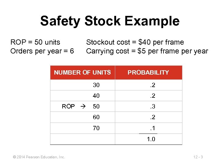Safety Stock Example ROP = 50 units Orders per year = 6 Stockout cost = $40 per frame Carrying cost = $5 per frame per year NUMBER OF UNITS PROBABILITY 30 40 . 2 50 . 3 60 . 2 70 ROP . 2 . 1 1. 0 © 2014 Pearson Education, Inc. 12 - 3

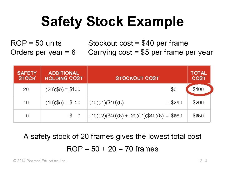Safety Stock Example ROP = 50 units Orders per year = 6 Stockout cost = $40 per frame Carrying cost = $5 per frame per year SAFETY STOCK ADDITIONAL HOLDING COST 20 (20)($5) = $100 10 (10)($5) = $ 50 0 $ 0 TOTAL COST STOCKOUT COST $0 $100 = $240 $290 (10)(. 2)($40)(6) + (20)(. 1)($40)(6) = $960 (10)(. 1)($40)(6) A safety stock of 20 frames gives the lowest total cost ROP = 50 + 20 = 70 frames © 2014 Pearson Education, Inc. 12 - 4

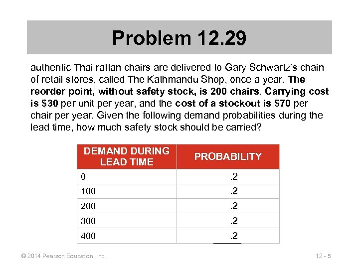Problem 12. 29 authentic Thai rattan chairs are delivered to Gary Schwartz’s chain of retail stores, called The Kathmandu Shop, once a year. The reorder point, without safety stock, is 200 chairs. Carrying cost is $30 per unit per year, and the cost of a stockout is $70 per chair per year. Given the following demand probabilities during the lead time, how much safety stock should be carried? DEMAND DURING LEAD TIME PROBABILITY 300 . 2. 2 400 . 2 0 100 200 © 2014 Pearson Education, Inc. 12 - 5

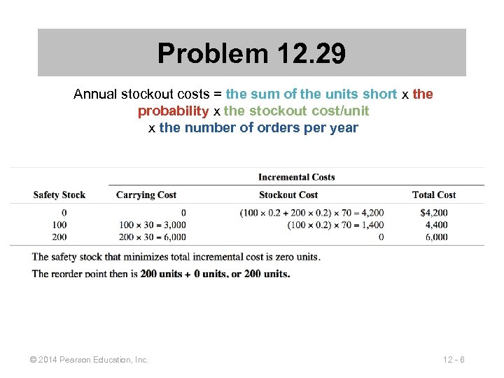Problem 12. 29 Annual stockout costs = the sum of the units short x the probability x the stockout cost/unit x the number of orders per year © 2014 Pearson Education, Inc. 12 - 6

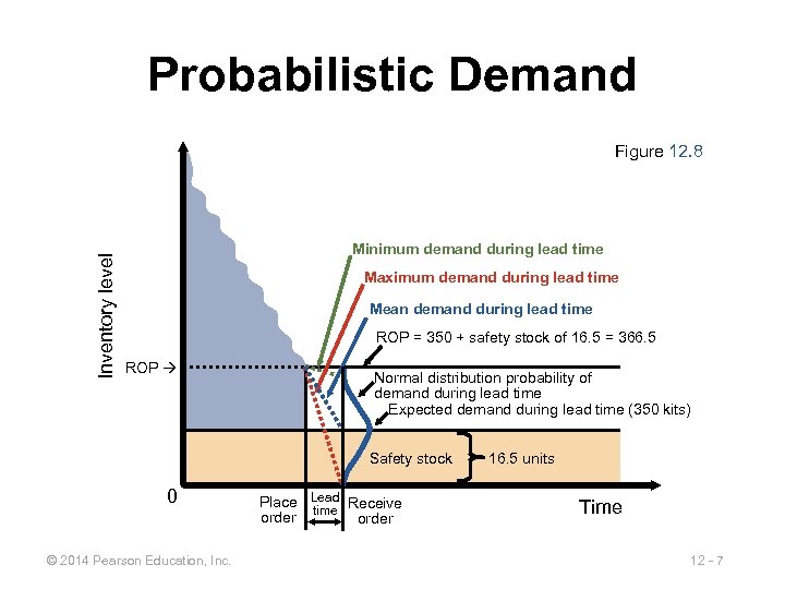Probabilistic Demand Inventory level Figure 12. 8 Minimum demand during lead time Maximum demand during lead time Mean demand during lead time ROP = 350 + safety stock of 16. 5 = 366. 5 ROP Normal distribution probability of demand during lead time Expected demand during lead time (350 kits) Safety stock 0 © 2014 Pearson Education, Inc. Place Lead Receive time order 16. 5 units Time 12 - 7

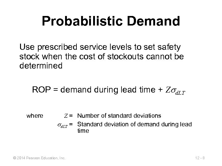Probabilistic Demand Use prescribed service levels to set safety stock when the cost of stockouts cannot be determined ROP = demand during lead time + Z d. LT where Z = Number of standard deviations d. LT = Standard deviation of demand during lead time © 2014 Pearson Education, Inc. 12 - 8

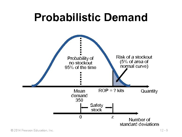Probabilistic Demand Risk of a stockout (5% of area of normal curve) Probability of no stockout 95% of the time Mean demand 350 0 © 2014 Pearson Education, Inc. ROP = ? kits Quantity Safety stock z Number of standard deviations 12 - 9

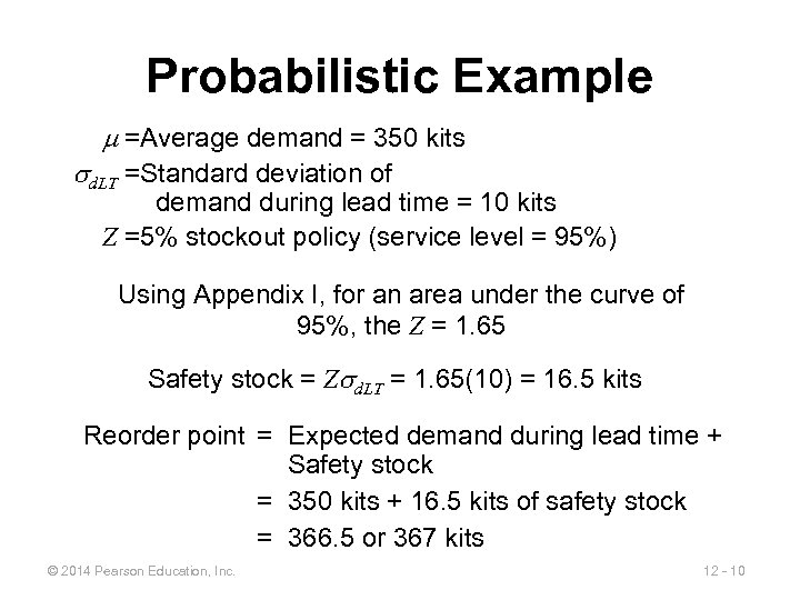Probabilistic Example m =Average demand = 350 kits d. LT =Standard deviation of demand during lead time = 10 kits Z =5% stockout policy (service level = 95%) Using Appendix I, for an area under the curve of 95%, the Z = 1. 65 Safety stock = Z d. LT = 1. 65(10) = 16. 5 kits Reorder point = Expected demand during lead time + Safety stock = 350 kits + 16. 5 kits of safety stock = 366. 5 or 367 kits © 2014 Pearson Education, Inc. 12 - 10

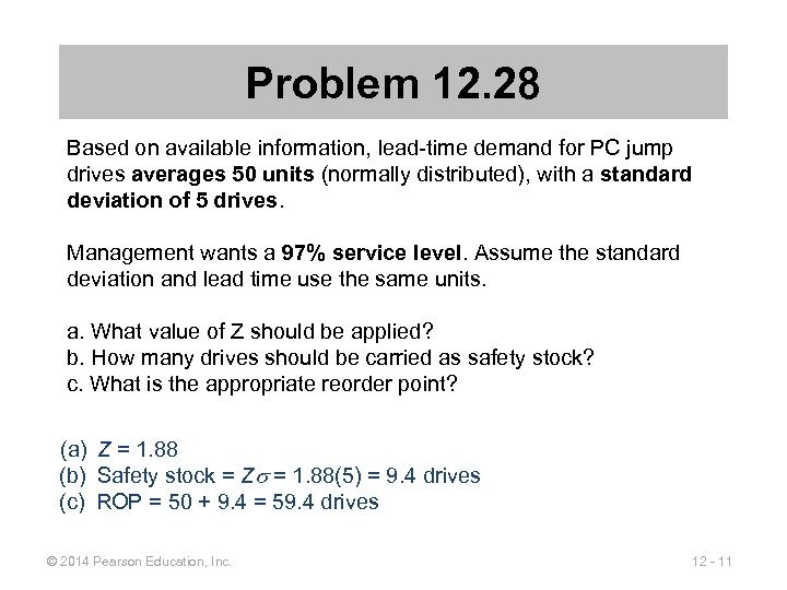Problem 12. 28 Based on available information, lead-time demand for PC jump drives averages 50 units (normally distributed), with a standard deviation of 5 drives. Management wants a 97% service level. Assume the standard deviation and lead time use the same units. a. What value of Z should be applied? b. How many drives should be carried as safety stock? c. What is the appropriate reorder point?   (a) Z = 1. 88 (b) Safety stock = Z = 1. 88(5) = 9. 4 drives (c) ROP = 50 + 9. 4 = 59. 4 drives © 2014 Pearson Education, Inc. 12 - 11

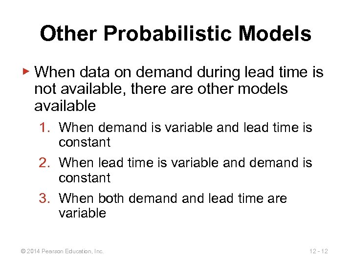Other Probabilistic Models ▶ When data on demand during lead time is not available, there are other models available 1. When demand is variable and lead time is constant 2. When lead time is variable and demand is constant 3. When both demand lead time are variable © 2014 Pearson Education, Inc. 12 - 12

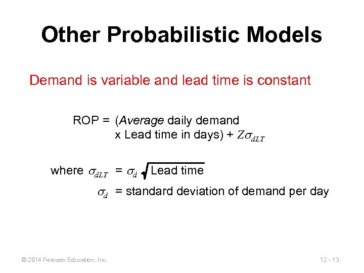Other Probabilistic Models Demand is variable and lead time is constant ROP = (Average daily demand x Lead time in days) + Z d. LT where d. LT = d Lead time d = standard deviation of demand per day © 2014 Pearson Education, Inc. 12 - 13

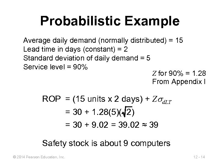Probabilistic Example Average daily demand (normally distributed) = 15 Lead time in days (constant) = 2 Standard deviation of daily demand = 5 Service level = 90% Z for 90% = 1. 28 From Appendix I ROP = (15 units x 2 days) + Z d. LT = 30 + 1. 28(5)( 2) = 30 + 9. 02 = 39. 02 ≈ 39 Safety stock is about 9 computers © 2014 Pearson Education, Inc. 12 - 14

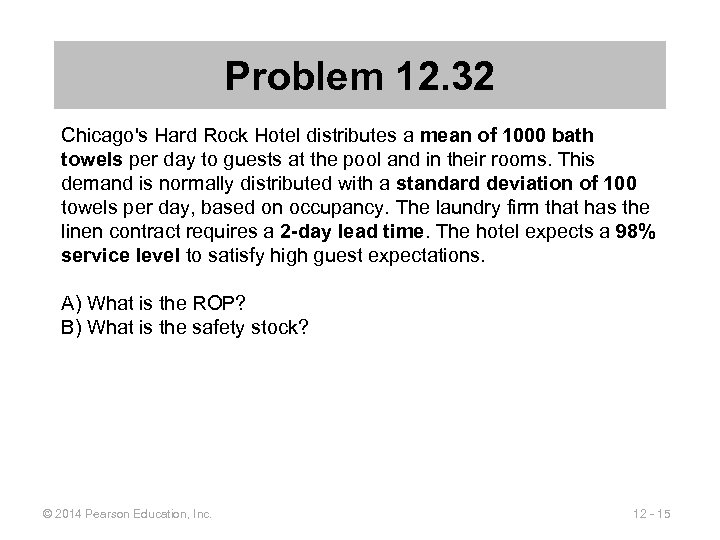Problem 12. 32 Chicago's Hard Rock Hotel distributes a mean of 1000 bath towels per day to guests at the pool and in their rooms. This demand is normally distributed with a standard deviation of 100 towels per day, based on occupancy. The laundry firm that has the linen contract requires a 2 -day lead time. The hotel expects a 98% service level to satisfy high guest expectations. A) What is the ROP? B) What is the safety stock? © 2014 Pearson Education, Inc. 12 - 15

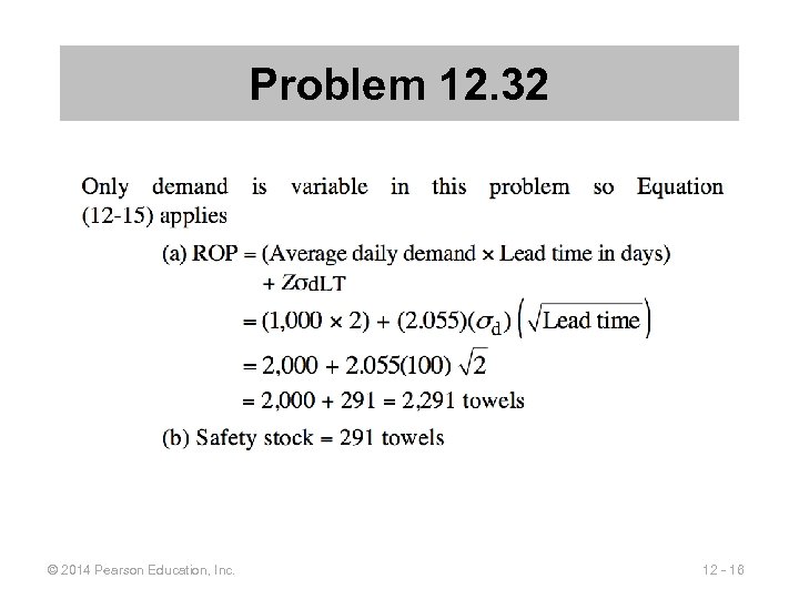Problem 12. 32 © 2014 Pearson Education, Inc. 12 - 16

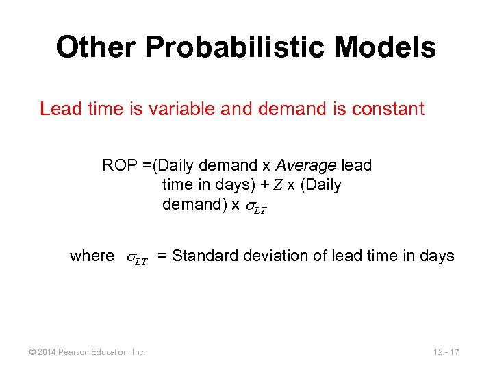Other Probabilistic Models Lead time is variable and demand is constant ROP =(Daily demand x Average lead time in days) + Z x (Daily demand) x LT where LT = Standard deviation of lead time in days © 2014 Pearson Education, Inc. 12 - 17

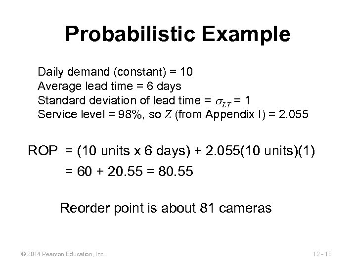Probabilistic Example Daily demand (constant) = 10 Average lead time = 6 days Standard deviation of lead time = LT = 1 Service level = 98%, so Z (from Appendix I) = 2. 055 ROP = (10 units x 6 days) + 2. 055(10 units)(1) = 60 + 20. 55 = 80. 55 Reorder point is about 81 cameras © 2014 Pearson Education, Inc. 12 - 18

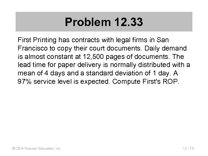Problem 12. 33 First Printing has contracts with legal firms in San Francisco to copy their court documents. Daily demand is almost constant at 12, 500 pages of documents. The lead time for paper delivery is normally distributed with a mean of 4 days and a standard deviation of 1 day. A 97% service level is expected. Compute First's ROP. © 2014 Pearson Education, Inc. 12 - 19

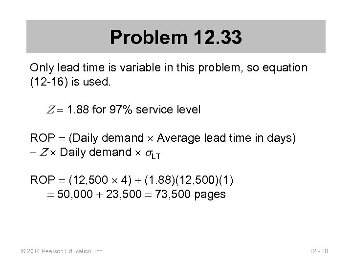Problem 12. 33 Only lead time is variable in this problem, so equation (12 -16) is used. 1. 88 for 97% service level ROP (Daily demand Average lead time in days) Daily demand LT ROP (12, 500 4) (1. 88)(12, 500)(1) 50, 000 23, 500 73, 500 pages © 2014 Pearson Education, Inc. 12 - 20

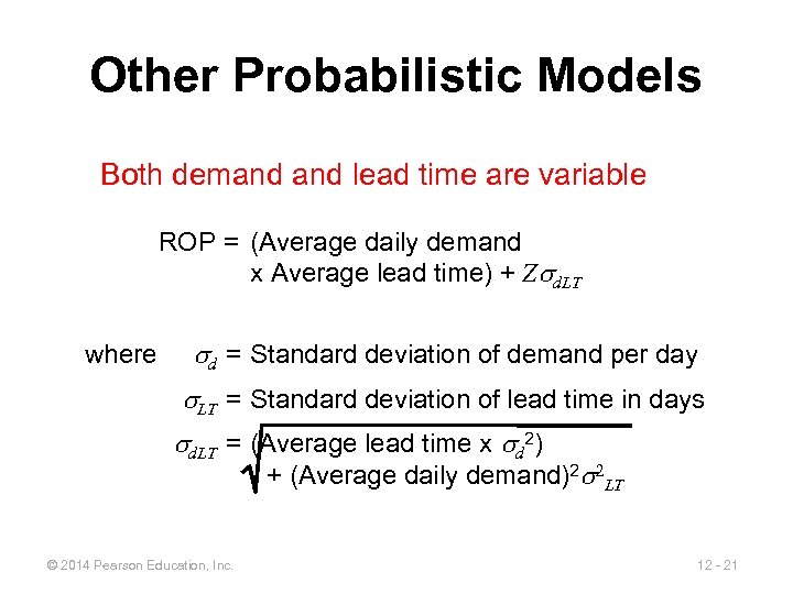Other Probabilistic Models Both demand lead time are variable ROP = (Average daily demand x Average lead time) + Z d. LT where d = Standard deviation of demand per day LT = Standard deviation of lead time in days d. LT = (Average lead time x d 2) + (Average daily demand)2 2 LT © 2014 Pearson Education, Inc. 12 - 21

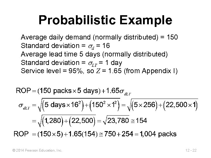Probabilistic Example Average daily demand (normally distributed) = 150 Standard deviation = d = 16 Average lead time 5 days (normally distributed) Standard deviation = LT = 1 day Service level = 95%, so Z = 1. 65 (from Appendix I) © 2014 Pearson Education, Inc. 12 - 22

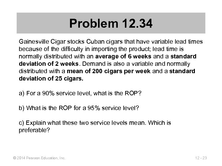Problem 12. 34 Gainesville Cigar stocks Cuban cigars that have variable lead times because of the difficulty in importing the product; lead time is normally distributed with an average of 6 weeks and a standard deviation of 2 weeks. Demand is also a variable and normally distributed with a mean of 200 cigars per week and a standard deviation of 25 cigars. a) For a 90% service level, what is the ROP? b) What is the ROP for a 95% service level? c) Explain what these two service levels mean. Which is preferable? © 2014 Pearson Education, Inc. 12 - 23

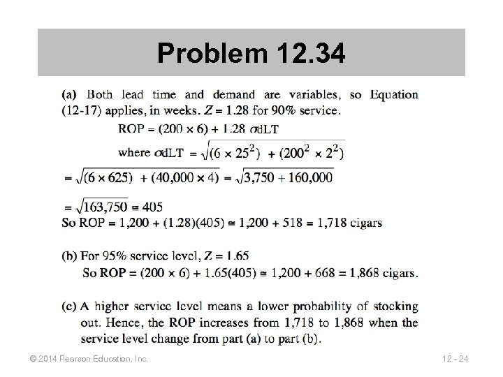Problem 12. 34 © 2014 Pearson Education, Inc. 12 - 24

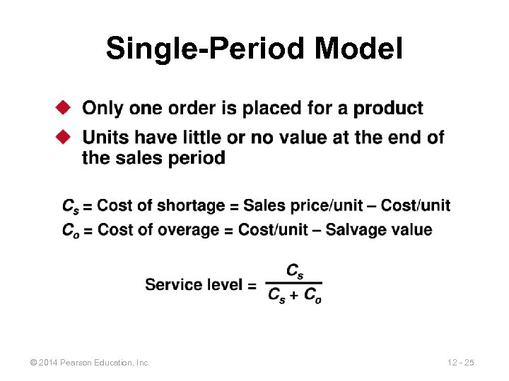Single-Period Model © 2014 Pearson Education, Inc. 12 - 25

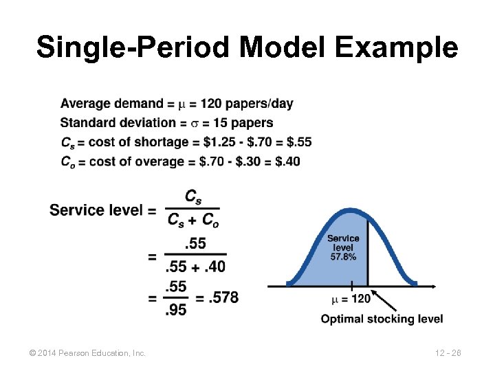Single-Period Model Example © 2014 Pearson Education, Inc. 12 - 26

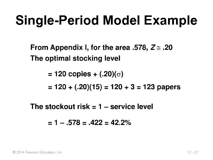Single-Period Model Example © 2014 Pearson Education, Inc. 12 - 27

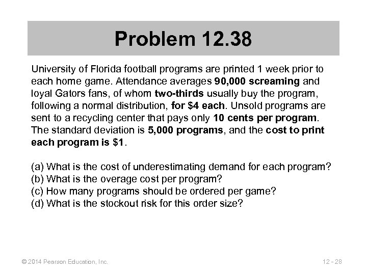Problem 12. 38 University of Florida football programs are printed 1 week prior to each home game. Attendance averages 90, 000 screaming and loyal Gators fans, of whom two-thirds usually buy the program, following a normal distribution, for $4 each. Unsold programs are sent to a recycling center that pays only 10 cents per program. The standard deviation is 5, 000 programs, and the cost to print each program is $1. (a) What is the cost of underestimating demand for each program? (b) What is the overage cost per program? (c) How many programs should be ordered per game? (d) What is the stockout risk for this order size? © 2014 Pearson Education, Inc. 12 - 28

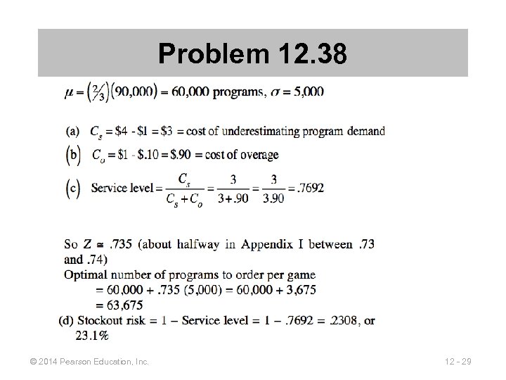Problem 12. 38 © 2014 Pearson Education, Inc. 12 - 29