Introduction to UNIX Working in a multi-user environment

Introduction to UNIX Working in a multi-user environment

What do you need to know? • This is not a course on computers • But you will need some UNIX for the exercises, and for your final project • You will also need to know some R to handle the exercises • But Gene. Publisher will handle R for you during the projects

What is UNIX? • UNIX is not just one operating system, but a collection of many different systems sharing a common interface • It has evolved alongside the internet and is geared toward multi-user environments, and big multiprocessors like our servers • At it’s heart, UNIX is a text-based operating system – that means a little typing is required • UNIX Lives! (Particularly Linux!)

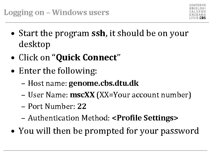Logging on – Windows users • Start the program ssh, it should be on your desktop • Click on “Quick Connect” • Enter the following: – Host name: genome. cbs. dtu. dk – User Name: msc. XX (XX=Your account number) – Port Number: 22 – Authentication Method: • You will then be prompted for your password

UNIX comes with a help system It depends on the program in question: – Either as a ‘man-page’ manual page using the command ‘man’ • Example: man less – Or through the ‘-h’ option • Example: acroread ‘-h’ By the way, the ‘man-pages’ are displayed using the program less, so you scroll with ‘k’ and ‘j’

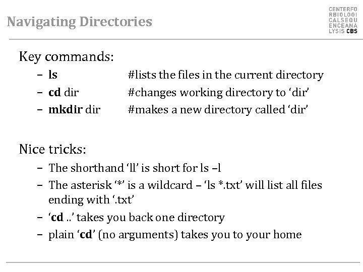Navigating Directories Key commands: – ls – cd dir – mkdir #lists the files in the current directory #changes working directory to ‘dir’ #makes a new directory called ‘dir’ Nice tricks: – The shorthand ‘ll’ is short for ls –l – The asterisk ‘*’ is a wildcard – ‘ls *. txt’ will list all files ending with ‘. txt’ – ‘cd. . ’ takes you back one directory – plain ‘cd’ (no arguments) takes you to your home

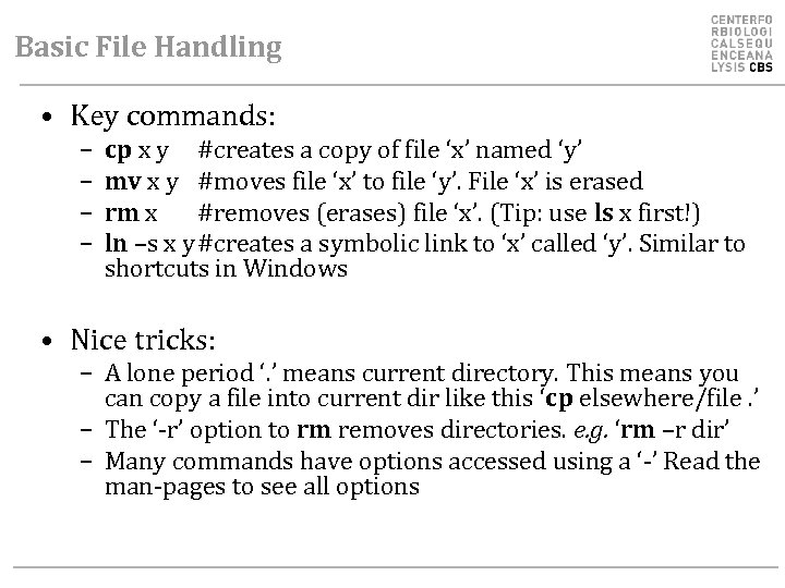Basic File Handling • Key commands: – – cp x y #creates a copy of file ‘x’ named ‘y’ mv x y #moves file ‘x’ to file ‘y’. File ‘x’ is erased rm x #removes (erases) file ‘x’. (Tip: use ls x first!) ln –s x y#creates a symbolic link to ‘x’ called ‘y’. Similar to shortcuts in Windows • Nice tricks: – A lone period ‘. ’ means current directory. This means you can copy a file into current dir like this ‘cp elsewhere/file. ’ – The ‘-r’ option to rm removes directories. e. g. ‘rm –r dir’ – Many commands have options accessed using a ‘-’ Read the man-pages to see all options

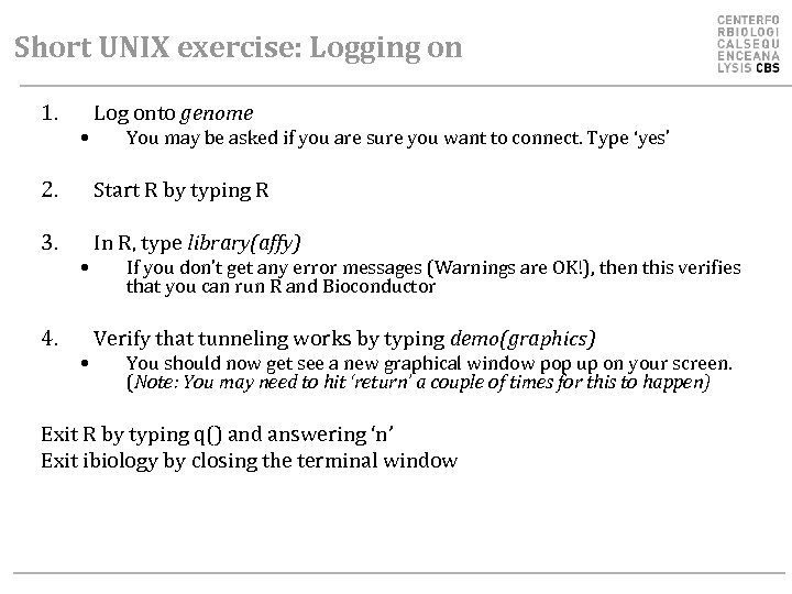Short UNIX exercise: Logging on 1. • Log onto genome You may be asked if you are sure you want to connect. Type ‘yes’ 2. Start R by typing R 3. In R, type library(affy) 4. • • If you don’t get any error messages (Warnings are OK!), then this verifies that you can run R and Bioconductor Verify that tunneling works by typing demo(graphics) You should now get see a new graphical window pop up on your screen. (Note: You may need to hit ‘return’ a couple of times for this to happen) Exit R by typing q() and answering ‘n’ Exit ibiology by closing the terminal window

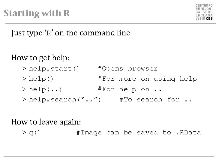Starting with R Just type ‘R’ on the command line How to get help: > > help. start() #Opens browser help() #For more on using help(. . ) #For help on. . help. search(“. . ”) #To search for. . How to leave again: > q() #Image can be saved to. RData

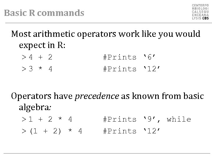Basic R commands Most arithmetic operators work like you would expect in R: >4 + 2 >3 * 4 #Prints ‘ 6’ #Prints ‘ 12’ Operators have precedence as known from basic algebra: >1 + 2 * 4 > (1 + 2) * 4 #Prints ‘ 9’, while #Prints ‘ 12’

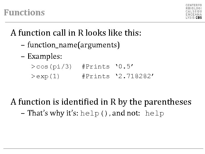Functions A function call in R looks like this: – function_name(arguments) – Examples: > cos(pi/3) > exp(1) #Prints ‘ 0. 5’ #Prints ‘ 2. 718282’ A function is identified in R by the parentheses – That’s why it’s: help(), and not: help

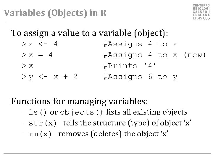Variables (Objects) in R To assign a value to a variable (object): > x <- 4 >x = 4 >x > y <- x + 2 #Assigns 4 to x (new) #Prints ‘ 4’ #Assigns 6 to y Functions for managing variables: – ls() or objects() lists all existing objects – str(x) tells the structure (type) of object ‘x’ – rm(x) removes (deletes) the object ‘x’

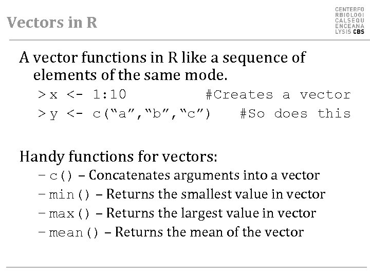Vectors in R A vector functions in R like a sequence of elements of the same mode. > x <- 1: 10 #Creates a vector > y <- c(“a”, “b”, “c”) #So does this Handy functions for vectors: – c() – Concatenates arguments into a vector – min() – Returns the smallest value in vector – max() – Returns the largest value in vector – mean() – Returns the mean of the vector

More on Vectors Elements in a vector can be accessed individually: > x[1] #Prints first element > x[1: 10] #Prints first 10 elements > x[c(1, 3)] #Prints element 1 and 3 Most functions expect one vector as argument, rather than individual numbers > mean(1, 2, 3) > mean(c(1, 2, 3)) #Replies ‘ 1’ #Replies ‘ 2’

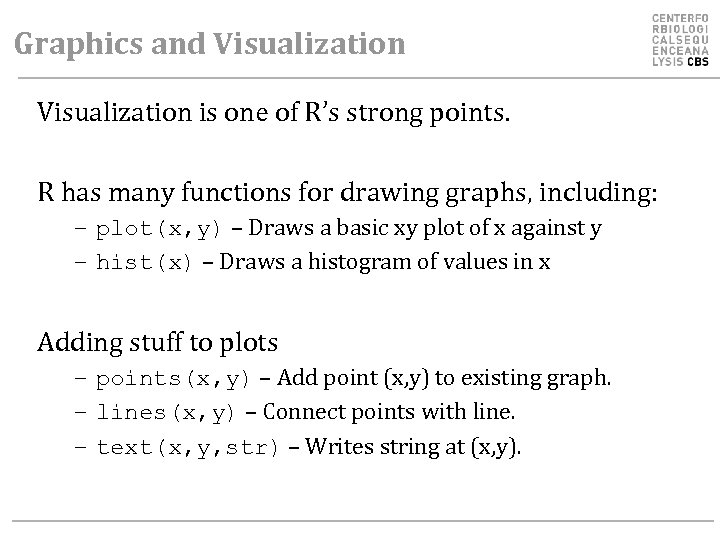Graphics and Visualization is one of R’s strong points. R has many functions for drawing graphs, including: – plot(x, y) – Draws a basic xy plot of x against y – hist(x) – Draws a histogram of values in x Adding stuff to plots – points(x, y) – Add point (x, y) to existing graph. – lines(x, y) – Connect points with line. – text(x, y, str) – Writes string at (x, y).

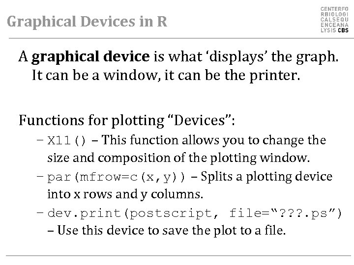Graphical Devices in R A graphical device is what ‘displays’ the graph. It can be a window, it can be the printer. Functions for plotting “Devices”: – X 11() – This function allows you to change the size and composition of the plotting window. – par(mfrow=c(x, y)) – Splits a plotting device into x rows and y columns. – dev. print(postscript, file=“? ? ? . ps”) – Use this device to save the plot to a file.