INTRODUCTION TO RISK MANAGEMENT Defense Resources Management Institute

INTRODUCTION TO RISK MANAGEMENT Defense Resources Management Institute Naval Postgraduate School Monterey, California

WHAT IS RISK?

DEFINITIONS I • Arabic - Fortuitous and favorable. • Greek - Fortuitous and neither favorable nor unfavorable. • Latin (risicum) - the challenge that a barrier reef presents to a sailor. • French (risque) - mainly negative connotation, but sometimes positive. • Oxford Dictionary - “. . . the chance of hazard, bad consequences, loss, etc. . ”

DEFINITIONS II • Economic risk - the chance of loss due to …. CHANCE lose money because…. . Random Occurrence • Business risk - the chance of loss associated with … • Market risk - the chance that a portfolio of investments can • Inflation risk - the danger that a general increase in prices. . . • Interest-rate risk - market risk due to interest rate fluctuations • Credit risk - the chance that of a default on a loan. . . BAD- the difficulty in selling a fixed asset. . . CONSEQUENCE Derivative risk - the chance of financial loss due to increased Sense of Loss volatility …. • Liquidity risk • • Cultural risk - the chance of loss because of product market …. . Hirschey & Pappas, Fundamentals of Managerial Economics Dryden Press, 1998

A LITTLE BIT OF PROBABILITY

PROBABILITY • It’s a number – it’s JUST A NUMBER! • It’s a number between 0 and 1 ( 0 ≤ P ≤ 1) • It quantifies the likelihood of an event • It’s a function of experience, judgment, subjective assessment, available data • It’s uses all information you think is relevant to the determination of the likelihood of occurrence of an event

Probability Rules Probability = 0 if “never/impossible” Probability = 1 if “always/certain” If we are collectively exhaustive and mutually exclusive then the probabilities over the outocmes SUM to 1.

Probability Rules • If mutually exclusive then : P(A or B) = P(A) + P(B) • If independent : P(A and B) = P(A) x P(B)

Probability from Data • Given data we can always derive approximate probabilities using relative frequency. • Relative frequency can be used as an estimate of the probability of the observed value • Taken all together, these can represent the underlying PROBABILITY DISTRUBUTION FUNCTION

Earthquakes

Frequency Table How Big? Richter Scale 1. 5 ≤ R < 2. 5 ≤ R < 3. 5 ≤ R < 4. 5 ≤ R < 5. 5 ≤ R < 6. 5 ≤ R < 7. 5 ≤ R < 8. 5 ≤ R < 9. 5 How Many? Number of Earthquakes 474 240 158 65 38 20 4 1

Relative Frequency Table How Big? Richter Scale 1. 5 ≤ R < 2. 5 ≤ R < 3. 5 ≤ R < 4. 5 ≤ R < 5. 5 ≤ R < 6. 5 ≤ R < 7. 5 ≤ R < 8. 5 ≤ R < 9. 5 How Many? Number of Earthquakes 0. 474 0. 240 0. 158 0. 065 0. 038 0. 020 0. 004 0. 001

Relative Frequency Histogram 0. 50 0. 474 0. 45 0. 40 0. 35 0. 30 0. 240 0. 25 0. 20 0. 158 0. 15 0. 10 0. 065 0. 038 0. 020 0. 004 0. 001 0. 00 [1. 5 - 2. 5) [2. 5 - 3. 5) [3. 5 - 4. 5) [4. 5 - 5. 5) [5. 5 - 6. 5) [6. 5 - 7. 5) [7. 5 - 8. 5) [8. 5 - 9. 5)

Prob. of an event = proportion of observations that corresponds to the event = percent of observations that corresponds to the event = portion of area of histogram that corresponds to the event

AN INVESTMENT DECISION • Planning for retirement • Two options for investment • Each has a track record, the historical rates-ofreturn over a specified time period • Each can be used to compute various statistics; e. g. , average rate-of-return, etc.

AN INVESTMENT DECISION Expected Value Std. Dev. Variance A 1 5. 00% 1. 25% 1. 5625 A 2 5. 70% 2. 75% 7. 5625

r n n r

What’s the likelihood of r<0 ? I don’t want a rate of return < 0! I want a rate of return > 0! What’s the likelihood of r<0 ?

THE FREQUENCY HISTOGRAM ( The “KEY to it ALL’’ ) • The relative frequency histogram over the outcomes contains all relevant information. • This information allows us to quantify risk. • This is provides our most powerful tool for risk management.

A QUANTITATIVE DEFINITION OF RISK

A QUANTITATIVE DEFINITION OF RISK Risk is a COMBINATION of the answers to three questions: (1) “What can go wrong? ” (2) “How likely is it to go wrong? ” (3) “If it does go wrong, what are the consequences? ” Adapted from S. Kaplan and B. John Garrick, “On the Quantitative Definition of Risk”, Risk Analysis, Vol. 1, no. 1, 1981

EXAMPLE: Hinterland Illegal Immigration What can go wrong? recession; depression; economic collapse How likely is it to go wrong? chances are 1 in a 10; a 10% chance; PF =. 10 If it does go wrong, what happens to Drmecia? large numbers of illegal immigrants ; increasing crime; failing social services; social unrest;

A QUANTITATIVE DEFINITION OF RISK What can go wrong? F Future scenario How likely is it to go wrong? PF Probability of F If it does go wrong, what are the consequences? Y Result due to F

THE ANSWER TO THE FIRST QUESTION 1. It all starts with the future scenario, F. 2. The F is uncertain so we need probability, PF. 3. F causes a result, an outcome of concern, Y. 4. Y is a function of F. We need to know this relation! The relation between Y and F is uncertain!!!

BEGINNING – MIDDLE – END F →X→Y F 1 F 2 F 3 … FK X 1 then X 2 then…. . XM THE “SYSTEM” Y 1 Y 2 Y 3 … YN F 1, F 2, … → X 1 then X 2 then… → Y 1, Y 2, …

EXAMPLE: Hinterland Illegal Immigration Illegal immigration is proportional to the ratio of per capita GDP. F = GDPD/pop. D GDPH/pop. H illegal immigration = Y G. H. Hanson (2009), “The Economics and Policy of Illegal Immigration in the U. S. ”, Washington, D. C. : Migration Policy Institute

THE ANSWER TO THE SECOND QUESTION PF X 1 then X 2 then…. . XM THE “SYSTEM” PY Distribution SIMULATION Probabilityfor → Math Model →Outcomes of Interest MODELING Probability Distribution for Future Scenarios

THE ANSWER TO THE SECOND QUESTION PY

THE ANSWER TO THE THIRD QUESTION What number of illegal immigrants do you most want to avoid? 10000; 1000000; 10000000; 20000000. HOW YOU FEEL (about the possible Y) = What outcome do you most prefer to avoid: minor economic strain; substantial strain; or collapse of government social/educational services? PREFERENCE

THE ANSWER TO THE THIRD QUESTION 1. It all starts with the future scenario, F. 2. The F is uncertain so we need probability, PF. 3. F causes a result, an outcome of concern, Y. 4. Y is a function of F. Given PF we can derive PY 5. How do you feel about the probable outcomes? Do you prefer to avoid some Y more than other Y?

THE ANSWER TO THE THIRD QUESTION • Preferences < = > value function < = > v(Y) (1) v(Y) > 0 if Y is “good” (2) v(Y) < 0 if Y is “bad” • Value Function Charcteristics (1) reference point [defining GAINS from LOSSES] (2) loss aversion [losses MORE IMPORTANT than GAINS] (3) decreasing marginal values

v(Y) Gains ( + ) concave Illegal Immigration Reference Point Losses ( - ) convex

A QUANTITATIVE DEFINITION OF RISK 1. It all starts with the future scenario, F. 2. The F is uncertain so we need probability, PF. 3. F causes a result, an outcome of concern, Y. 4. Y is a function of F. Given PF we can derive PY 5. Your preference info, v(Y), defines the PIECE! is the LAST consequences!

Probability Distribution (Outcome) AND Decision Maker Preferences AND PY AND v(Y)

Hinterland Economy Collapse Prob. of Economic Collapse PF F g(F) Number of Illegal Immigrants g(F) PY Y Prob. Dist. Illegal Immigrants Risk v(Y) How does Drmecia “feel” about the Y?

SPECIAL CASE OF PREFERENCE v(Y) Y

SPECIAL CASE OF PREFERENCE v(Y) Y In the limit the weight we assign to all outcomes <=> a loss tends to - ∞. In this case risk is very simple to quantify risk. “I can’t bear the thought of experiencing loss! “ “Experiencing loss would be a catastrophe!”

ASSESSING THE RISK PY 0. 1 v(Y) 0. 2 0. 3 0. 4 + 0. 5 0. 6 0. 7 0. 8 - 0. 9 1. 0

ASSESSING THE RISK PY 0. 1 v(Y) 0. 2 0. 3 0. 4 0. 5 0. 6 0. 7 0. 8 0. 9 1. 0

ASSESSING THE RISK (SPECIAL CASE) RISK = P{ Y correspond to loss } RISK = P{ Y ≥ reference point } RISK = P{ unacceptable Y } RISK = P{ Y you prefer to avoid }

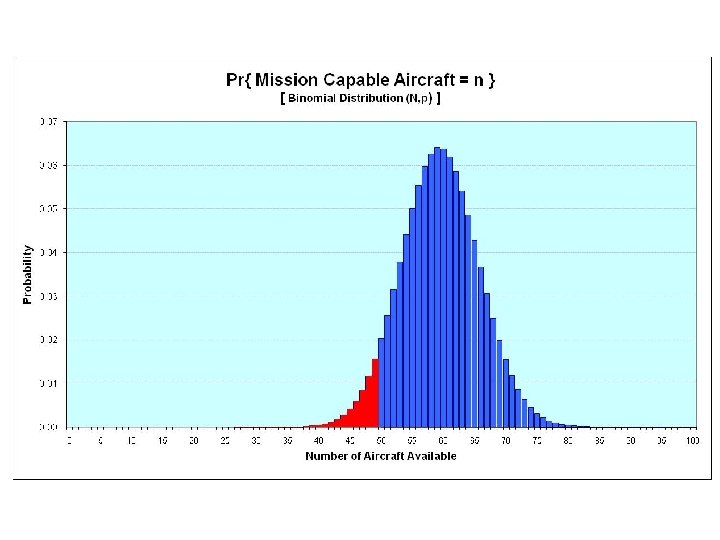
Who uses this stuff? . . . . OVERALL C-RATING System for Readiness: C-1 = MAE > 89% P{not capable} ≤ 0. 11 C-2 = MAE 80 -89% 0. 11 ≤ P{not capable} ≤ 0. 20 C-3 = MAE 70 -79% 0. 21 ≤ P{not capable} ≤ 0. 30 C-4 = MAE 50 -69% 0. 31 ≤ P{not capable} ≤ 0. 50 C-5 = MAE < 50% 0. 50 ≤ P{not capable} Senate Armed Services Committee, terminology used in arguments before the committee, Feb. 1997 AR 220 – 1 (2010), AFI 10 -201 (2006), SORTS (US Department of Defense)

A QUANTITATIVE APPROACH TO RISK MANAGEMENT

The History of Risk Management • 1950 B. C. – Code of Hamurabi – formalization of bottomry contracts containing a risk premium for chance of loss of ships and cargo. • 750 B. C. – Greece – the use of bottomry contracts. • 1285 A. D. – King Edward - forbids use of soft coal in kilns to manage air pollution in London. • 1583 A. D. – 1 st life insurance policy issued in England. • 19 th and 20 th century – water and garbage sanitation, building codes, fire codes, boiler inspections, railroads, steamboats, autos. • 1959 A. D. – H. Markowitz, stock portfolio diversification.

RISK MANAGEMENT PROCESS Identify Risks What can go wrong F? What is F and PF? Assess Risks What are the outcomes [Y, and PY]? What are the consequences, v(Y)? Prevent Implement Monitor Mitigate Negotiate What is the risk [quantified]? Management Action

Tools of Risk Management • Prevention. • Mitigation. • Hedging. • Diversification.

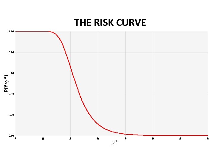
ASSESSING THE RISK Definition depends on a reference point. National policy often specifies a reference point. Not everyone has the same reference point. THE ≥ y* } CURVE Why not plot P{ Y RISKversus y*, for any y* ?

Determining the Outcome Distribution • theoretical derivation • direct assessment • simulation your own data Generating

EARTHQUAKES Number of earthquakes Earthquake cost Size of earthquake VARIABLE Cost per earthquake Total cost Program Cost FIXED Earthquake policy

1. 00 0. 652 0. 11 0. 012 P{ Total Cost ≥ 0. 002 } 0. 00 y*

0. 10 0. 08 A 1 : Do Nothing 0. 06 0. 04 0. 02 30 40 50 60 70 20 10 10 10 0 0. 00 0. 10 0. 08 0. 06 A 2 : New Building Codes 0. 04 0. 02 0. 00 0. 10 0. 08 0. 06 A 3 : Retro-Fit & New Codes 0. 04 0. 02 0. 00

P{ Total Cost ≥ x } 1. 00 0. 80 The 0. 60 RISK CURVES 0. 40 compared 0. 20 70 60 50 40 30 20 10 0 0. 00

1. 00 0. 80 0. 652 A 1 (red) 0. 60 A 2 (blue) 0. 40 0. 328 A 3 (green) 0. 20 0. 065 70 60 50 40 30 20 10 0 0. 00

ACCEPTABLE RISK “The perennial question free people ask with regard to defense is: ‘How much is enough? ’ To this there can be no precise answer. A country’s security is a function of the DEGREE OF RISK A COUNTRY IS WILLING TO ACCEPT. ” Hitch & Mc. Kean, The Economics of Defense in the Nuclear Age, Atheneum, 1986

ACCEPTABLE RISK Risk Too Risky Acceptable Risk Proposed Budget Required Budget Cost

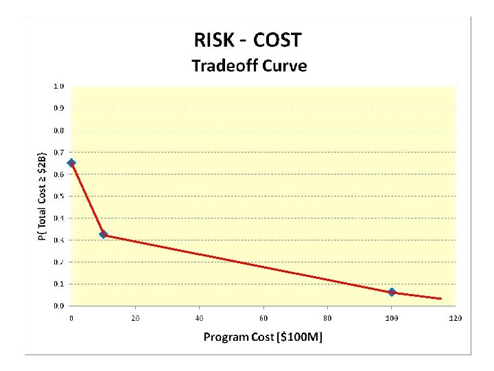
Who uses this stuff? . . . . Ultimately, policy makers must decide how much the United States is willing to pay to lower the risks associated with deploying forces abroad. But some might argue that defense planners occasionally focus on absolute requirements – the minimum number of forces that they believe will meet Do. D’s military needs – without fully weighing the relative risks and costs of alternative levels. Moving U. S. Forces: Options for Strategic Mobility Congressional Budget Office, Feb. 1997

Who uses this stuff? . . . . “Our armed forces remain capable, within an acceptable level of risk, of meeting the demands of our strategy. ” Maj. Gen. John J. Maher, Vice Director for Operations, Joint Staff: testimony before House National Security readiness subcommittee, Feb. 1997

Who uses this stuff? . . . . “Computer security is basically risk management. ” “…. Managers have to decide what they are trying to protect and how much they are willing to spend, both in cost and convenience, to defend it. ” Stephen H. Wildstrom, review of the book “Secrets and Lies by Bruce Schneier, Businessweek Sept. 2000

Who uses this stuff? . . . . “…we continue to believe the federal government can benefit from risk management. ” “…. An effective risk management approach includes a threat assessment, a vulnerability assessment and a criticality assessment. . . ” Raymond J. Decker, Director, Defense Capabilities and Management, GAO, Testimony before the Senate Committee on Governmental Affairs Oct. 2001

RISK MANAGEMENT Risk old new Cost

RISK MANAGEMENT Risk new Proposed Budget Cost

RISK MANAGEMENT Risk Acceptable Risk new Cost

APPLICATION I ENTERPRISE BUSINESS RISK

Error P =. 02 P(uncorrected) = 0. 1 Reconciliation Check Data Entry P(corrected) = 0. 9 P(error) = 0. 2 Correct P =. 18 Correct P =. 80 P(correct) = 0. 8 SECNAV M-5200. 35 March 2007

End User Define Needs, prepare Purchase Requisition Form Direct or Indirect/Reimb. ? DIR. Forward to ASA INDIR. Forward to SPFA Purchase Agent Sponsored Program Admin. Support NO YES ASA reviews PR, confirms funds, obtains approval SPFA Reviews PR Funds Available, etc. ? NO Funds Available, etc. ? YES SPFA assigns PR number and form to PA

End User ASA /OA will Assign req. , number and task Purchaser Purchase Agent Sponsored Program Admin. Support Clarify requirements with end user NO Purchaser reviews for completeness of documentation YES All required info. present and adequate to make procurement? Screen request for mandatory sources of supply, prohibited or special items, and authority to buy Buy from mandatory source or go open market?

End User Receive ordered items and sign acknowledging Purchase Agent Sponsored Program Admin. Support STOP YES Place order with source, direct delivery point, and provide estimated delivery date Receive order (if delivery point) Order complete and accurate? NO Reconcile with vendor

P =. 6561 What can go wrong? 0. 9 How likely is it to go wrong? NO ERROR Receipt Review ERROR P =. 1 0. 9 ASA 0. 1 P =ERROR. 0729 Screen Request 0. 9 0. 1 Reimburse Or Direct Funds Purchaser P =ERROR. 081 0. 9 0. 1 P =. 09 ERROR SPFA P ERROR =. 1 0. 1 P =. 3439

P =. 69255 0. 9 NO ERROR Receipt Review ERROR P =. 05 0. 9 ASA 0. 1 P =. 07695 ERROR Screen Request 0. 95 Reimburse Or Direct Funds 0. 1 P =. 0855 ERROR Purchaser 0. 95 0. 1 P =ERROR. 095 SPFA 0. 05 P =. 05 ERROR P =. 30745

P =. 8145 0. 95 NO ERROR Receipt Review ERROR P =. 05 0. 95 ASA 0. 05 P =ERROR. 04287 Screen Request 0. 95 Reimburse Or Direct Funds 0. 05 ERROR P =. 0451 Purchaser 0. 95 0. 05 ERROR P =. 0475 SPFA 0. 05 P =. 05 ERROR P =. 1855

P =. 9606 0. 95 P =. 01 Receipt Review ERROR 0. 01 0. 99 ASA NO ERROR 0. 01 P ERROR =. 009703 Screen Request 0. 99 Reimburse Or Direct Funds 0. 01 P ERROR =. 009801 Purchaser 0. 99 0. 01 ERROR P =. 0099 SPFA 0. 01 ERROR P =. 01 P =. 0394

APPLICATION II COST RISK ASSESSMENT

ESTIMATING SHIPBOARD HELICOPTER O&M COSTS Life-cycle cost estimates for the helicopter are needed. The cost analysis staff is organized into four groups, one each for the four main components of the lifecycle cost: (1) R&D; (2) Procurement; (3) Operations and Maintenance; and (4) Salvage/Residual. As leader of the O&M cost estimating group you have decided to use a factor cost estimates since: 1. Relevant O&M cost data produce reliable CERs for the three components of the O&M cost [POL, Parts, and “Other”] as functions of the procurement cost. 2. The helicopter is a recently developed model and procurement cost is expected to be $3. 7 million (+/- 3%). 3. Why not just use an O&M cost factor approach: annual O&M cost = 10% of acquisition cost?

POL[$/hr] = 112. 84 + 30. 16 × ACQ + error Parts[$/hr] = -84. 96 + 57. 21 × ACQ + error Other[$/hr] = 45. 21 + 10. 12 × ACQ + error

PROBABILISTIC COST ESTIMATING Future explanatory variable is not always known with certainty Cost estimate is a RANDOM VARIABLE y=a+bx+e Intercept is subject to estimation error There always is the model residual error Slope coefficient is subject to estimation error

PROBABILISTIC COST ESTIMATING What is the most appropriate distribution function? What is the resulting distribution function? y=a+bx+e What is the most appropriate distribution function?

PROBABILISTIC COST ESTIMATING ? y=a+bx+e ?

c. POL = a 1 + b 1×ACQ + e 1 c. Parts = a 2 + b 2×ACQ + e 2 c. Other = a 3 + b 3×ACQ + e 3 CO, M&S = [c. POL + c. Parts + cother ] × H

Annual O, M & S Cost : CASE 1 0. 000 $164 K ≤ 0. 000 CO, M&S ≤ $676 0. 000 0. 000 9 E-06 8 E-06 7 E-06 Values in Thousands 6 E-06 5 E-06 4 E-06 3 E-06 2 E-06 1 E-06 0. 000

Annual O, M & S Cost : CASE 2 0. 000 $164 K ≤ 0. 000 CO, M&S ≤ $672 0. 000 0. 000 9 E-06 8 E-06 7 E-06 Values in Thousands 6 E-06 5 E-06 4 E-06 3 E-06 2 E-06 1 E-06 0. 000

Annual O, M & S Cost : CASE 3 0. 000 $158 K ≤ 0. 000 CO, M&S ≤ $511 0. 000 0. 000 9 E-06 8 E-06 7 E-06 Values in Thousands 6 E-06 5 E-06 4 E-06 3 E-06 2 E-06 1 E-06 0. 000

Annual O, M & S Cost : CASE 4 0. 000 $190 K ≤ 0. 000 CO, M&S ≤ $463 K 0. 000 0. 000 9 E-06 8. 5 E-06 8 E-06 7. 5 E-06 7 E-06 6. 5 E-06 Values in Thousands 6 E-06 5. 5 E-06 4 E-06 3. 5 E-06 3 E-06 2. 5 E-06 2 E-06 1. 5 E-06 1 E-06 0. 000

APPLICATION III PROJECT MANAGEMENT

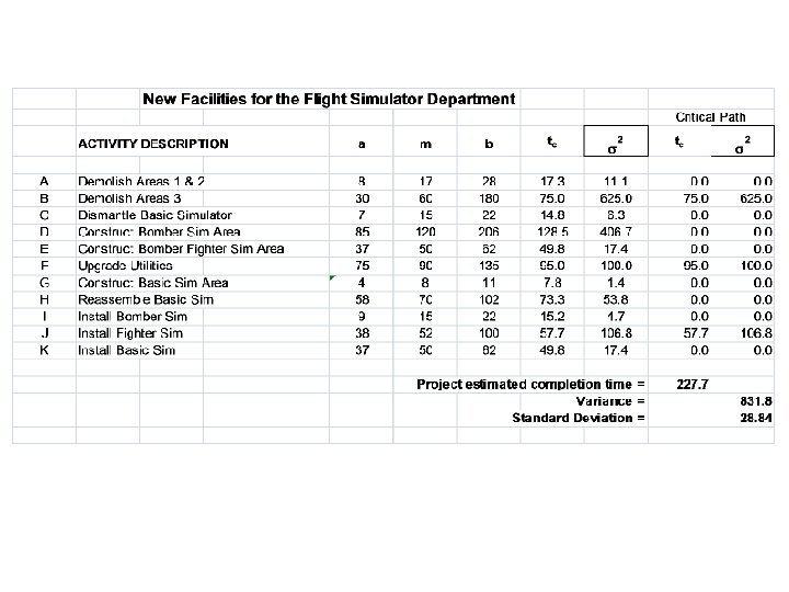
FACILITIES FOR THE FLIGHT SIMULATOR DEPARTMENT (ACTIVITIES, TIME ESTIMATES, AND DEPENDENCIES)

P = 0. 482

P = 0. 048

SUMMARY • RISK is a factor in every decision with significant uncertainty • RISK is a combination of the answers to 3 questions – what can go wrong? – how likely is it to go wrong? – if it does go wrong, what are the consequences?

SUMMARY • RISK is quantified using PROBABILITY. – use it to express the riskiness an alternative. – use it to find the least risky alternative. • THINK about the RISK vs COST tradeoff curve.

SUMMARY • MANAGING RISK requires the information provided by the tradeoff curve! – THINK about where you want to be on the curve. – THINK about changing the tradeoff curve! • USE THE MODEL to help find how to change things!