Introduction to Planarity Test W L Hsu 1

Introduction to Planarity Test W. L. Hsu 1

Plane Graph l A plane graph is a graph drawn in the plane in such a way that no two edges intersect – Except at a vertex to which they are both incident l A planar graph is one which is isomorphic to a plane graph – Namely, it has a plane embedding 2

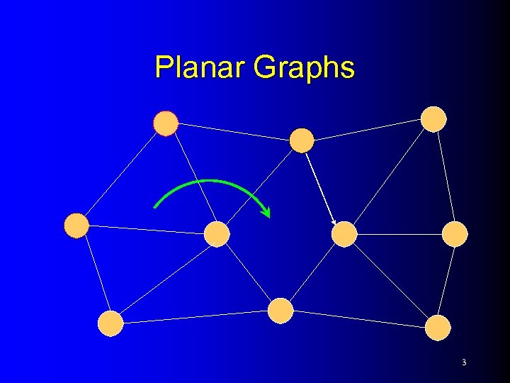Planar Graphs 3

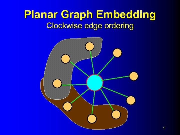Planar Graph Embedding Clockwise edge ordering 4

Issues in Planarity Test If you can find a planar embedding, then the graph is planar. l How do you determine if a graph is not planar? l This is the more difficult part of many recognition algorithm, namely, deciding when a graph “does not” belong to a class l – Get a certificate for non-planar graphs – Or alternatively, you have tried all possible ways but still fail to embed the graph in the plane (proof by exhaustion) – Use counting argument 5

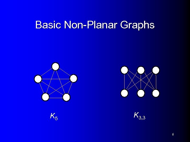Basic Non-Planar Graphs K 5 K 3, 3 6

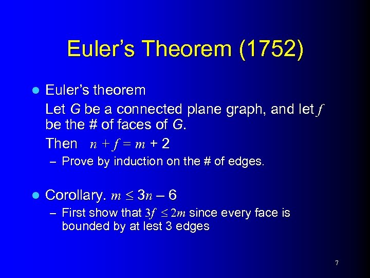Euler’s Theorem (1752) l Euler’s theorem Let G be a connected plane graph, and let f be the # of faces of G. Then n + f = m + 2 – Prove by induction on the # of edges. l Corollary. m 3 n – 6 – First show that 3 f 2 m since every face is bounded by at lest 3 edges 7

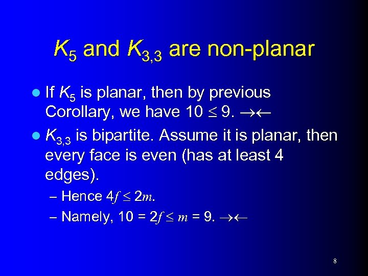K 5 and K 3, 3 are non-planar l If K 5 is planar, then by previous Corollary, we have 10 9. l K 3, 3 is bipartite. Assume it is planar, then every face is even (has at least 4 edges). – Hence 4 f 2 m. – Namely, 10 = 2 f m = 9. 8

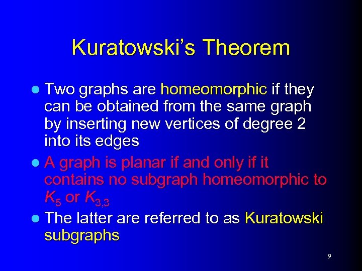Kuratowski’s Theorem l Two graphs are homeomorphic if they can be obtained from the same graph by inserting new vertices of degree 2 into its edges l A graph is planar if and only if it contains no subgraph homeomorphic to K 5 or K 3, 3 l The latter are referred to as Kuratowski subgraphs 9

Planarity Test 10

How do you draw a planar graph without regret ? l This means that, besides keeping the current embedding planar, your embedding can also keep future options open. l You will have to design an embedding “scheme” rather than obtain a “physical” (實體的 ) embedding 11

Prior Results l 1 st approach – Hopcroft and Tarjan [1974], first O(m) time. – PATH ADDITION l 2 nd approach – – l Lempel, Even and Cederbaum[1967], O(n 2) time VERTEX ADDITION st-numbering, consecutive ones testing Booth and Lueker [1976] used PQ-trees to test the consecutive ones property in O(m+n) time 3 rd approach – Shih and Hsu [1999] used PC-trees for recognition and embedding. – EDGE ADDITION 12

A Brief Intro. to the Vertex Addition Approach of LEC 13

Vertex Addition Approach of LEC Keep the current partial planar graph connected 2. Keep those non-added vertices a connected subgraph (i. e. in the same face). 3. Apply a consecutive ones test every time a new vertex is added 1. 14

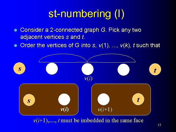st-numbering (I) Consider a 2 -connected graph G. Pick any two adjacent vertices s and t. l Order the vertices of G into s, v(1), . . . , v(k), t such that l s t v(i) t s v(i) v(i+1), …, t must be imbedded in the same face 15

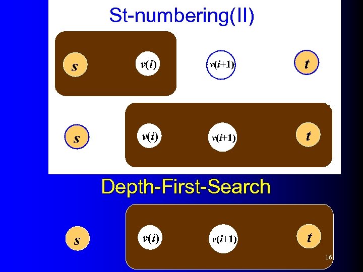St-numbering(II) s v(i) v(i+1) t Depth-First-Search s v(i) v(i+1) t 16

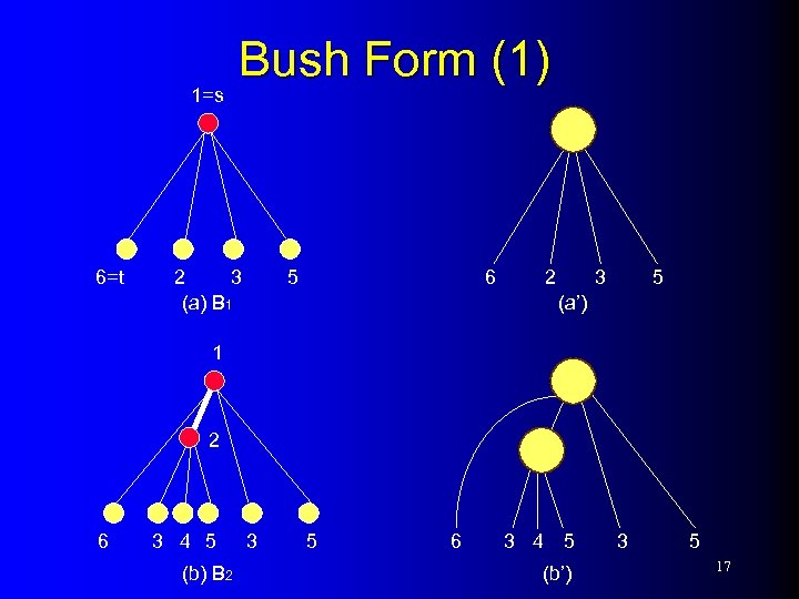Bush Form (1) 1=s 6=t 2 3 (a) B 1 6 5 2 3 5 (a’) 1 2 6 3 4 5 (b) B 2 3 5 6 3 4 5 (b’) 3 5 17

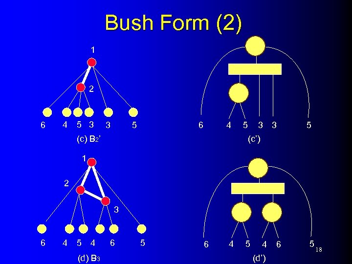Bush Form (2) 1 2 6 4 5 3 3 5 (c’) (c) B 2’ 1 2 3 6 4 5 4 (d) B 3 6 5 6 4 5 4 (d’) 6 5 18

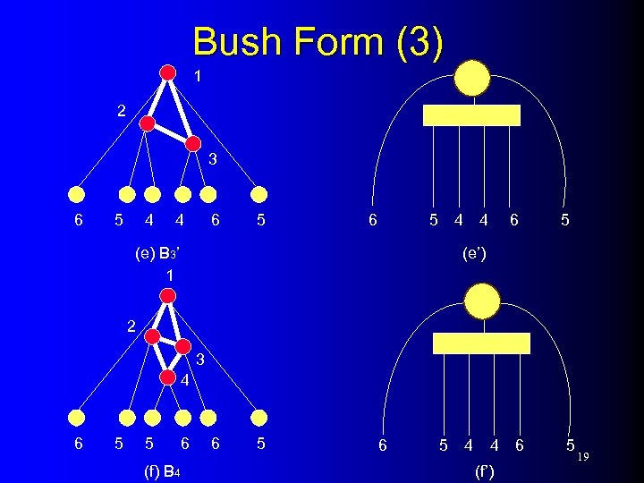Bush Form (3) 1 2 3 6 5 4 4 (e) B 3’ 1 6 5 (e’) 2 3 4 6 5 5 (f) B 4 6 6 5 4 4 (f’) 6 5 19

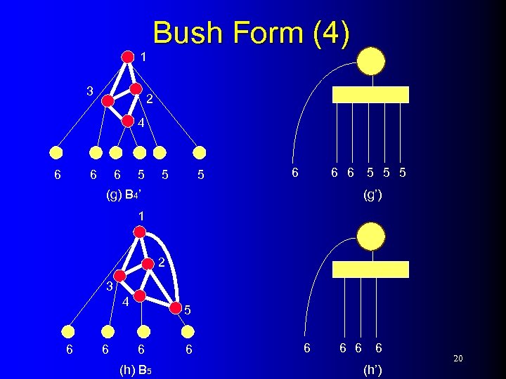1 3 Bush Form (4) 2 4 6 6 6 5 5 5 (g’) (g) B 4’ 1 2 3 4 6 6 5 6 (h) B 5 6 6 6 (h’) 20

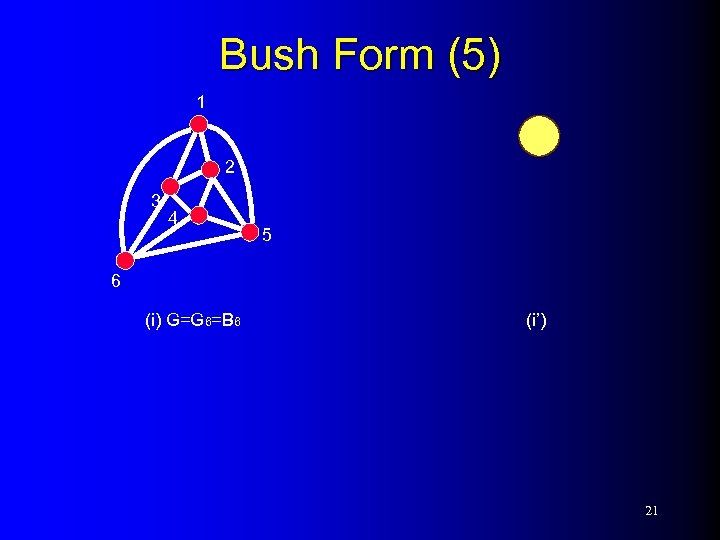Bush Form (5) 1 2 3 4 5 6 (i) G=G 6=B 6 (i’) 21

Introducing PQ-Trees 22

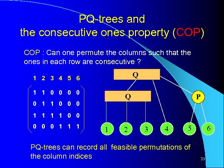PQ-trees and the consecutive ones property (COP) COP : Can one permute the columns such that the ones in each row are consecutive ? Q 1 2 3 4 5 6 1 1 0 0 Q 0 1 1 0 0 0 P 1 1 0 0 0 1 1 2 3 4 5 PQ-trees can record all feasible permutations of the column indices 6 23

Linear time algorithm on PQ-trees l [1974] Booth and Lueker presented a linear time algorithm for the COP test based on PQ-trees – Process the matrix one row at a time l PQ-tree can also be used to yield a linear time algorithm for interval graph recognition and planar graph recognition. 24

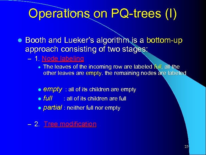Operations on PQ-trees (I) l Booth and Lueker’s algorithm is a bottom-up approach consisting of two stages: – 1. Node labeling l The leaves of the incoming row are labeled full, all the other leaves are empty. the remaining nodes are labeled empty : all of its children are empty l full : all of its children are full l partial : neither full nor empty l – 2. Tree modification 25

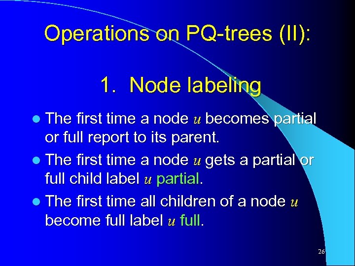Operations on PQ-trees (II): 1. Node labeling l The first time a node u becomes partial or full report to its parent. l The first time a node u gets a partial or full child label u partial. l The first time all children of a node u become full label u full. 26

Operations on PQ-trees (III): 2. Tree modification Need to modify the current tree so that all the incoming columns can be arranged consecutively. l Modify the subtree of every partial node l – At each iteration, modify the subtree of a partial node starting from the lowest level of the tree l The subtree modification is based on 9 templates of subtree structures. 27

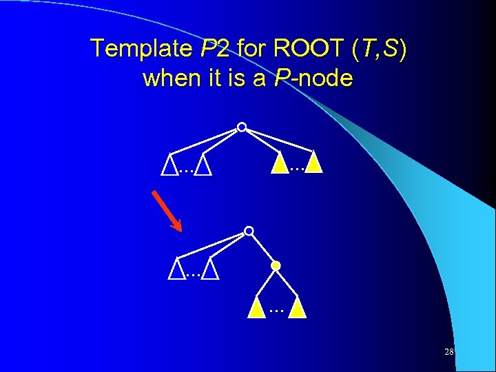Template P 2 for ROOT (T, S) when it is a P-node. . . 28

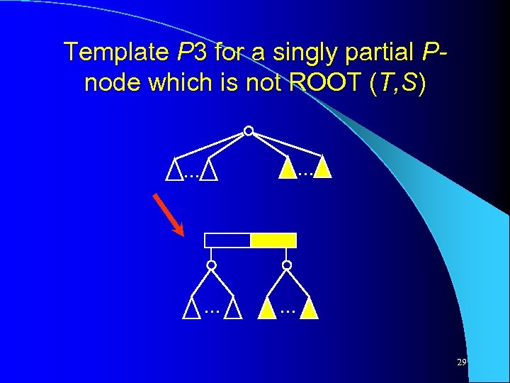Template P 3 for a singly partial Pnode which is not ROOT (T, S). . . 29

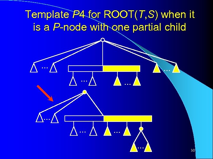Template P 4 for ROOT(T, S) when it is a P-node with one partial child . . . 30

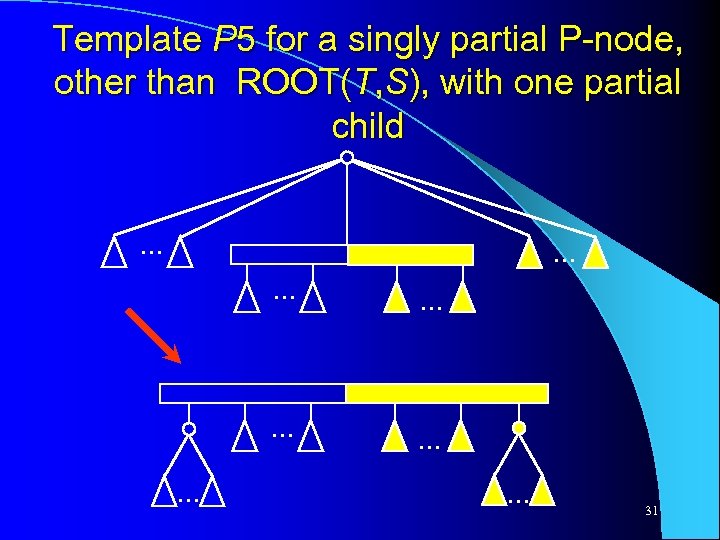Template P 5 for a singly partial P-node, other than ROOT(T, S), with one partial child. . . 31

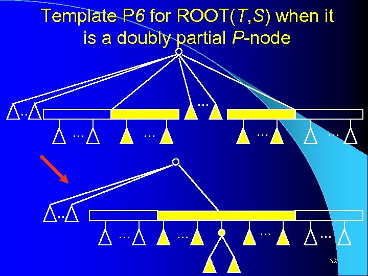Template P 6 for ROOT(T, S) when it is a doubly partial P-node. . . . 32

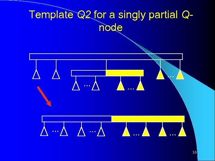Template Q 2 for a singly partial Qnode . . 33

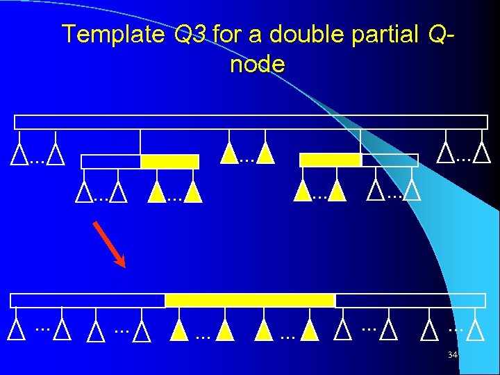Template Q 3 for a double partial Qnode . . 34

Time complexity of the original PQ-tree operations Node labeling takes time proportional to the number of incoming columns. l Subtree modification needs to change many parent-children relationships l – use amortized analysis to argue that it takes constant time at every iteration. – this analysis is quite involved. l Does not render a direct algorithm for testing the circular ones property – Complement a row 35