INTRODUCTION TO OPERATIONS RESEARCH Dynamic Programming DYNAMIC

INTRODUCTION TO OPERATIONS RESEARCH Dynamic Programming

DYNAMIC PROGRAMMING Decomposes a problem into a series of subproblems v Builds up correct solutions to larger and larger subproblems v v Examples of Dynamic Programming: Coins v Binomial v Scheduling v v Knapsack Problem v Viterbi Algorithm v Sequence Alignment

DYNAMIC PROGRAMMING v DP is a method for solving certain kind of problems v DP can be applied when the solution of a problem includes solutions to subproblems v We need to find a recursive formula for the solution v We can recursively solve subproblems, starting from the trivial case, and save their solutions in memory v In the end we’ll get the solution of the whole problem 3

PROPERTIES OF DYNAMIC PROGRAMMING v Simple Subproblems v We should be able to break the original problem to smaller subproblems that have the same structure v Optimal Substructure of the problems v The solution to the problem must be a composition of subproblem solutions v Subproblem Overlap v Optimal subproblems to unrelated problems can contain subproblems in common 4

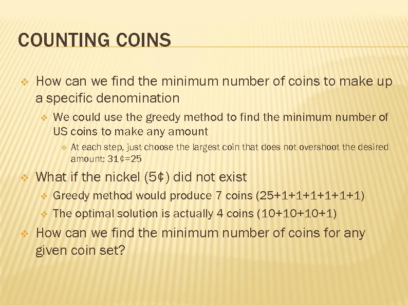COUNTING COINS v How can we find the minimum number of coins to make up a specific denomination v We could use the greedy method to find the minimum number of US coins to make any amount v v What if the nickel (5¢) did not exist v v v At each step, just choose the largest coin that does not overshoot the desired amount: 31¢=25 Greedy method would produce 7 coins (25+1+1+1) The optimal solution is actually 4 coins (10+10+10+1) How can we find the minimum number of coins for any given coin set?

COIN SET FOR EXAMPLES v For the following examples, we will assume coins in the following denominations: 1¢ 5¢ 10¢ 21¢ 25¢ v We’ll use 63¢ as our goal

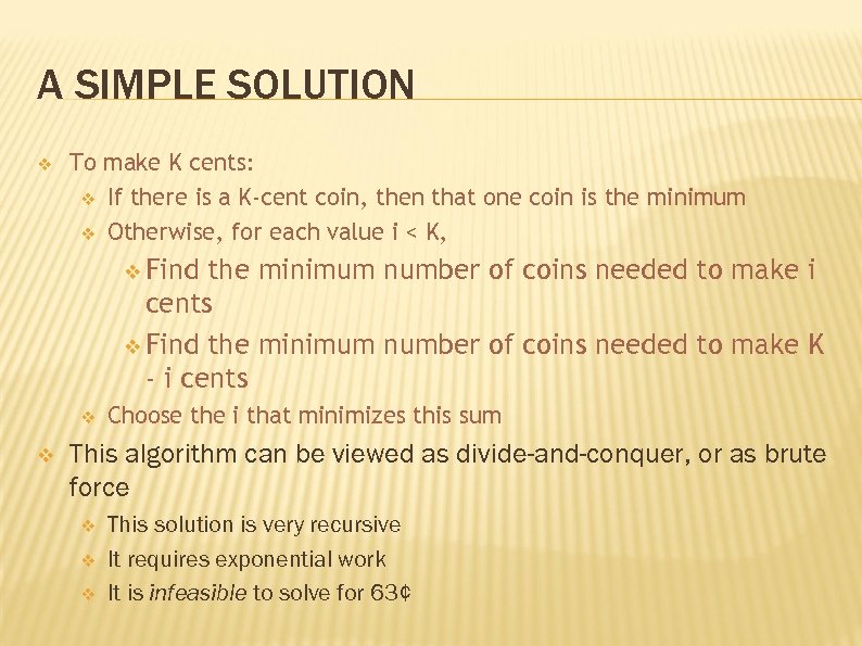A SIMPLE SOLUTION v To make K cents: v If there is a K-cent coin, then that one coin is the minimum v Otherwise, for each value i < K, v Find the minimum number of coins needed to make i cents v Find the minimum number of coins needed to make K - i cents v v Choose the i that minimizes this sum This algorithm can be viewed as divide-and-conquer, or as brute force v v v This solution is very recursive It requires exponential work It is infeasible to solve for 63¢

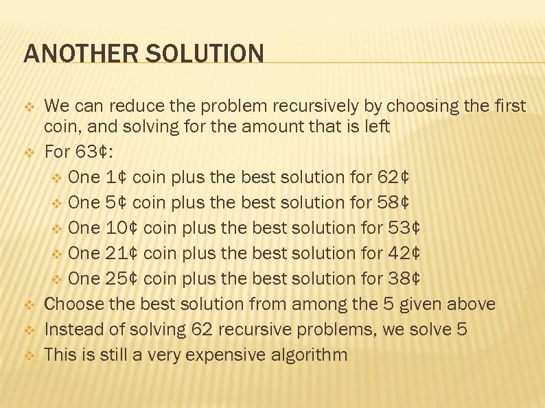ANOTHER SOLUTION v v v We can reduce the problem recursively by choosing the first coin, and solving for the amount that is left For 63¢: v One 1¢ coin plus the best solution for 62¢ v One 5¢ coin plus the best solution for 58¢ v One 10¢ coin plus the best solution for 53¢ v One 21¢ coin plus the best solution for 42¢ v One 25¢ coin plus the best solution for 38¢ Choose the best solution from among the 5 given above Instead of solving 62 recursive problems, we solve 5 This is still a very expensive algorithm

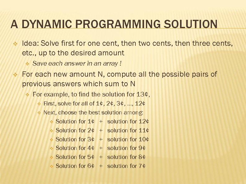A DYNAMIC PROGRAMMING SOLUTION v Idea: Solve first for one cent, then two cents, then three cents, etc. , up to the desired amount v v Save each answer in an array ! For each new amount N, compute all the possible pairs of previous answers which sum to N v For example, to find the solution for 13¢, v v First, solve for all of 1¢, 2¢, 3¢, . . . , 12¢ Next, choose the best solution among: v Solution for 1¢ + solution for 12¢ v Solution for 2¢ + solution for 11¢ v Solution for 3¢ + solution for 10¢ v Solution for 4¢ + solution for 9¢ v Solution for 5¢ + solution for 8¢ v Solution for 6¢ + solution for 7¢

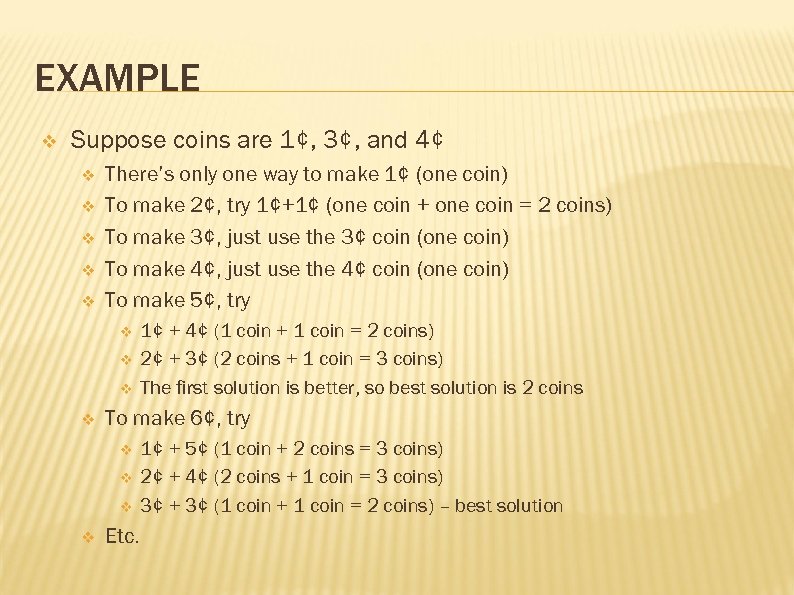EXAMPLE v Suppose coins are 1¢, 3¢, and 4¢ v v v There’s only one way to make 1¢ (one coin) To make 2¢, try 1¢+1¢ (one coin + one coin = 2 coins) To make 3¢, just use the 3¢ coin (one coin) To make 4¢, just use the 4¢ coin (one coin) To make 5¢, try v v To make 6¢, try v v 1¢ + 4¢ (1 coin + 1 coin = 2 coins) 2¢ + 3¢ (2 coins + 1 coin = 3 coins) The first solution is better, so best solution is 2 coins Etc. 1¢ + 5¢ (1 coin + 2 coins = 3 coins) 2¢ + 4¢ (2 coins + 1 coin = 3 coins) 3¢ + 3¢ (1 coin + 1 coin = 2 coins) – best solution

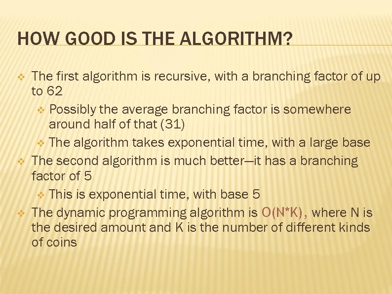HOW GOOD IS THE ALGORITHM? v v v The first algorithm is recursive, with a branching factor of up to 62 v Possibly the average branching factor is somewhere around half of that (31) v The algorithm takes exponential time, with a large base The second algorithm is much better—it has a branching factor of 5 v This is exponential time, with base 5 The dynamic programming algorithm is O(N*K), where N is the desired amount and K is the number of different kinds of coins

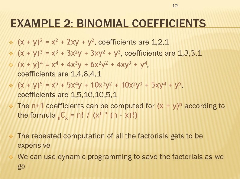12 EXAMPLE 2: BINOMIAL COEFFICIENTS v v v v (x + y)2 = x 2 + 2 xy + y 2, coefficients are 1, 2, 1 (x + y)3 = x 3 + 3 x 2 y + 3 xy 2 + y 3, coefficients are 1, 3, 3, 1 (x + y)4 = x 4 + 4 x 3 y + 6 x 2 y 2 + 4 xy 3 + y 4, coefficients are 1, 4, 6, 4, 1 (x + y)5 = x 5 + 5 x 4 y + 10 x 3 y 2 + 10 x 2 y 3 + 5 xy 4 + y 5, coefficients are 1, 5, 10, 5, 1 The n+1 coefficients can be computed for (x + y)n according to the formula n. Cx = n! / (x! * (n – x)!) The repeated computation of all the factorials gets to be expensive We can use dynamic programming to save the factorials as we go

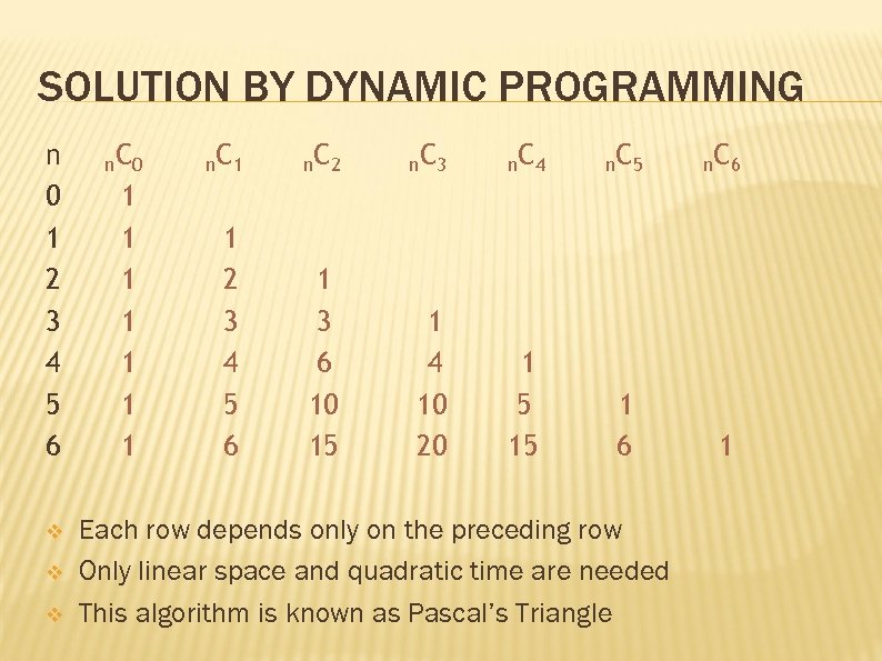SOLUTION BY DYNAMIC PROGRAMMING n 0 1 2 3 4 5 6 v v v n C 0 1 1 1 1 n C 2 n C 3 n C 4 n C 5 n C 6 1 2 3 4 5 6 1 3 6 10 15 1 4 10 20 1 5 15 1 6 1 Each row depends only on the preceding row Only linear space and quadratic time are needed This algorithm is known as Pascal’s Triangle

THE PRINCIPLE OF OPTIMALITY v v v Dynamic programming is a technique for finding an optimal solution The principle of optimality applies if the optimal solution to a problem always contains optimal solutions to all subproblems Example: Consider the problem of making N¢ with the fewest number of coins v Eithere is an N¢ coin, or v The set of coins making up an optimal solution for N¢ can be divided into two nonempty subsets, n 1¢ and n 2¢ v If either subset, n 1¢ or n 2¢, can be made with fewer coins, then clearly N¢ can be made with fewer coins

THE PRINCIPLE OF OPTIMALITY v The principle of optimality holds if v v The principle of optimality does not say v v If you have optimal solutions to all subproblems then you can combine them to get an optimal solution Example: In US coinage, v v Every optimal solution to a problem contains optimal solutions to all subproblems The optimal solution to 7¢ is 5¢ + 1¢, and The optimal solution to 6¢ is 5¢ + 1¢, but The optimal solution to 13¢ is not 5¢ + 1¢ + 5¢ + 1¢ But there is some way of dividing up 13¢ into subsets with optimal solutions (say, 11¢ + 2¢) that will give an optimal solution for 13¢ v Hence, the principle of optimality holds for this problem

DYNAMIC PROGRAMMING v Dynamic programming relies on working “from the bottom up” and saving the results of solving simpler problems v v v Dynamic programming solutions can often be quite complex and tricky Dynamic programming is used for optimization problems, especially ones that would otherwise take exponential time v v These solutions to simpler problems are then used to compute the solution to more complex problems Only problems that satisfy the principle of optimality are suitable for dynamic programming solutions Since exponential time is unacceptable for all but the smallest problems, dynamic programming is sometimes essential

WEIGHTED INTERVAL SCHEDULING v Problem v v scheduling a lecture hall each request has start time, end time, value goal: maximize value Basic idea v v sort requests by end time calculate p( request ) v v optimal schedule for requests 1. . n: v v v the next previous request that does not overlap if n part of optimal solution: optimal schedule for p( n ) and n else: optimal schedule for n-1 use sub solutions to build up complete solution

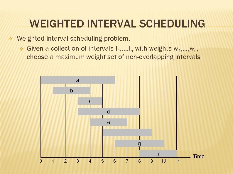WEIGHTED INTERVAL SCHEDULING v Weighted interval scheduling problem. v Given a collection of intervals I 1, …, In with weights w 1, …, wn, choose a maximum weight set of non-overlapping intervals a b c d e f g h 0 1 2 3 4 5 6 7 8 9 10 11 Time

WEIGHTED INTERVAL SCHEDULING Weighted interval scheduling problem. v Given a collection of intervals I 1, …, In with weights w 1, …, wn, choose a maximum weight set of non-overlapping intervals v p(j) = largest index i < j such that job i is compatible with j v Previous job p(1) = 0 p(2) = 0 p(3) = 1 p(4) = 0 p(5) = 3 p(6) = 3 w 1 = 2 1 w 2 = 4 2 w 3 = 4 3 4 w 4 = 7 w 5 = 2 5 w 6 = 1 6 0 1 2 3 4 5 6 7 8 9 10 11 Time

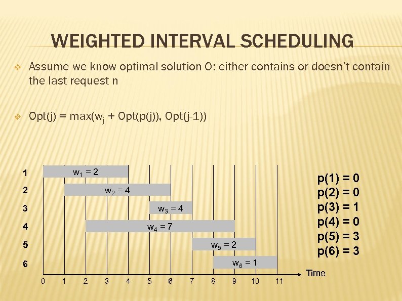WEIGHTED INTERVAL SCHEDULING v Assume we know optimal solution O: either contains or doesn’t contain the last request n v Opt(j) = max(wj + Opt(p(j)), Opt(j-1)) w 1 = 2 1 p(1) = 0 p(2) = 0 p(3) = 1 p(4) = 0 p(5) = 3 p(6) = 3 w 2 = 4 2 w 3 = 4 3 w 4 = 7 4 w 5 = 2 5 w 6 = 1 6 0 1 2 3 4 5 6 7 8 9 10 11 Time

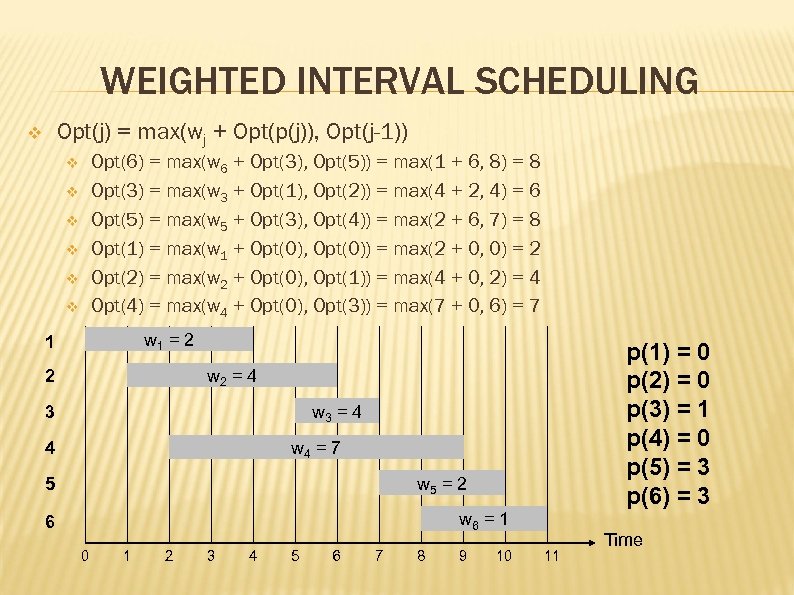WEIGHTED INTERVAL SCHEDULING Opt(j) = max(wj + Opt(p(j)), Opt(j-1)) v Opt(6) = max(w 6 + Opt(3), Opt(5)) = max(1 + 6, 8) = 8 Opt(3) = max(w 3 + Opt(1), Opt(2)) = max(4 + 2, 4) = 6 Opt(5) = max(w 5 + Opt(3), Opt(4)) = max(2 + 6, 7) = 8 Opt(1) = max(w 1 + Opt(0), Opt(0)) = max(2 + 0, 0) = 2 Opt(2) = max(w 2 + Opt(0), Opt(1)) = max(4 + 0, 2) = 4 Opt(4) = max(w 4 + Opt(0), Opt(3)) = max(7 + 0, 6) = 7 v v v w 1 = 2 1 p(1) = 0 p(2) = 0 p(3) = 1 p(4) = 0 p(5) = 3 p(6) = 3 w 2 = 4 2 w 3 = 4 3 w 4 = 7 4 w 5 = 2 5 w 6 = 1 6 0 1 2 3 4 5 6 7 8 9 10 11 Time

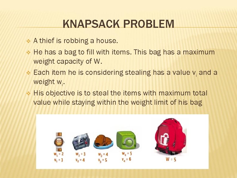KNAPSACK PROBLEM v v A thief is robbing a house. He has a bag to fill with items. This bag has a maximum weight capacity of W. Each item he is considering stealing has a value vi and a weight wi. His objective is to steal the items with maximum total value while staying within the weight limit of his bag

KNAPSACK PROBLEM v v In this case, what would a sub-problem be? Does a solution for item n include the solution for item n-1? Assume we know optimal solution O: either contains or doesn’t contain the last item n v It Does v v v It Doesn’t v v Add value of item n (vn) to the total value O must contain an optimal solution to the problem consisting of item n 1 and total weight W – wn O is equal to the optimal solution to the problem consisting of item n-1 and total weight W If w < wi then Opt(i, w) = Opt(i – 1, w) otherwise Opt(i, w) = max(Opt(i – 1, w), vi + Opt(i -1, w – wi))

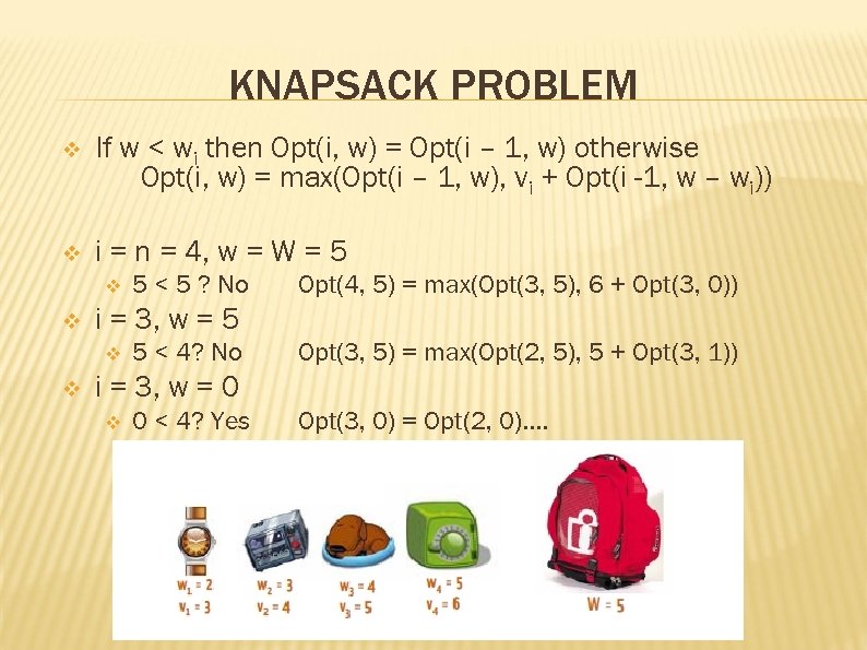KNAPSACK PROBLEM v If w < wi then Opt(i, w) = Opt(i – 1, w) otherwise Opt(i, w) = max(Opt(i – 1, w), vi + Opt(i -1, w – wi)) v i = n = 4, w = W = 5 v v Opt(4, 5) = max(Opt(3, 5), 6 + Opt(3, 0)) i = 3, w = 5 v v 5 < 5 ? No 5 < 4? No Opt(3, 5) = max(Opt(2, 5), 5 + Opt(3, 1)) i = 3, w = 0 v 0 < 4? Yes Opt(3, 0) = Opt(2, 0). .

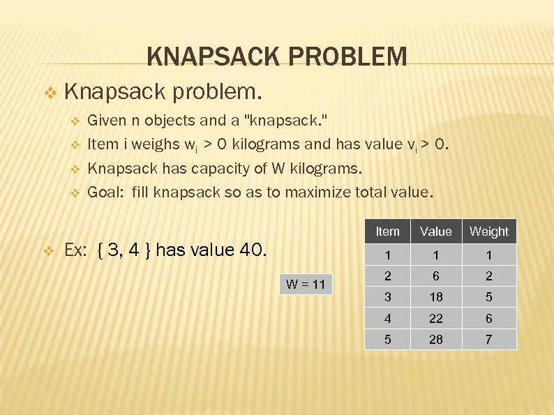KNAPSACK PROBLEM v Knapsack problem. v Given n objects and a "knapsack. " v Item i weighs wi > 0 kilograms and has value vi > 0. v Knapsack has capacity of W kilograms. v Goal: fill knapsack so as to maximize total value. v Item W = 11 Weight 1 Ex: { 3, 4 } has value 40. Value 1 1 2 6 2 3 18 5 4 22 6 5 28 7

KNAPSACK PROBLEM v Def. OPT(i) = max profit subset of items 1, …, i. v Case 1: OPT does not select item i. v OPT selects best of { 1, 2, …, i-1 } v Case 2: OPT selects item i. v accepting item i does not immediately imply that we will have to reject other items v without knowing what other items were selected before i, we don't even know if we have enough room for I Conclusion. Need more sub-problems! v

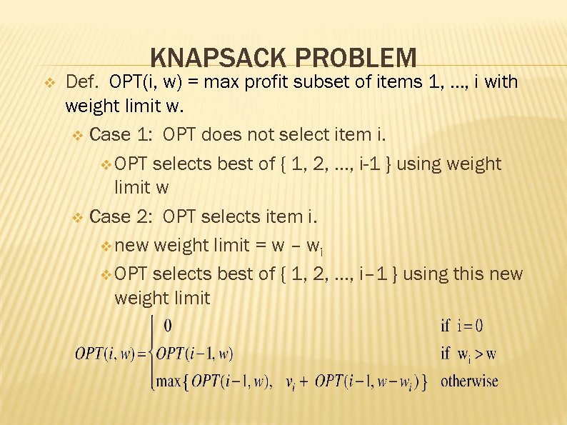KNAPSACK PROBLEM v Def. OPT(i, w) = max profit subset of items 1, …, i with weight limit w. v Case 1: OPT does not select item i. v OPT selects best of { 1, 2, …, i-1 } using weight limit w v Case 2: OPT selects item i. v new weight limit = w – wi v OPT selects best of { 1, 2, …, i– 1 } using this new weight limit

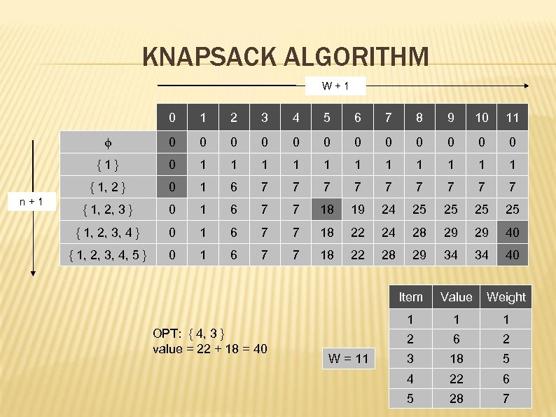KNAPSACK ALGORITHM W+1 0 2 3 4 5 6 7 8 9 10 11 0 0 0 {1} 0 1 1 1 { 1, 2 } n+1 1 0 1 6 7 7 7 7 7 { 1, 2, 3 } 0 1 6 7 7 18 19 24 25 25 { 1, 2, 3, 4 } 0 1 6 7 7 18 22 24 28 29 29 40 { 1, 2, 3, 4, 5 } 0 1 6 7 7 18 22 28 29 34 34 40 Item 1 1 2 W = 11 Weight 1 OPT: { 4, 3 } value = 22 + 18 = 40 Value 6 2 3 18 5 4 22 6 5 28 7