Introduction to mixed models Ulf Olsson Unit of

Introduction to mixed models Ulf Olsson Unit of Applied Statistics and Mathematics 1

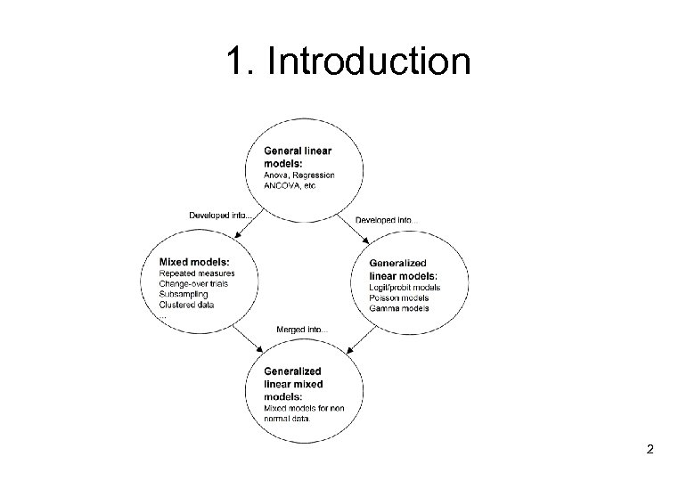1. Introduction 2

2. General linear models (GLM) But. . . I'm not using any model. I'm only doing a few t tests. 3

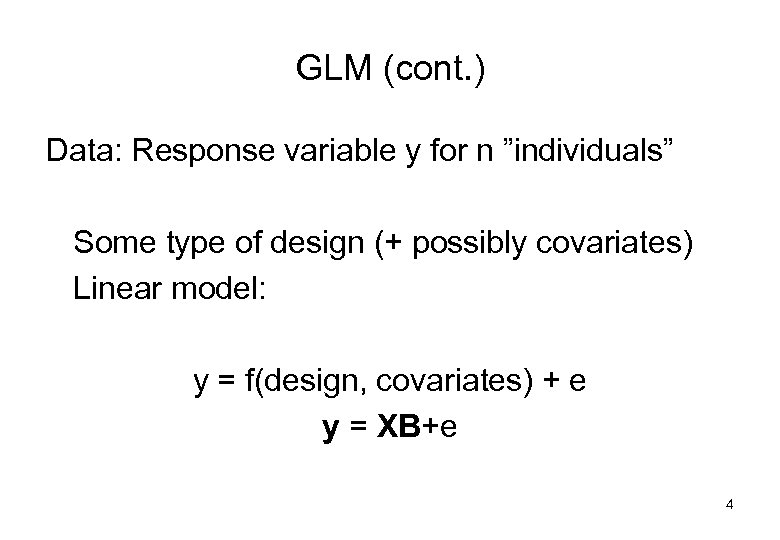GLM (cont. ) Data: Response variable y for n ”individuals” Some type of design (+ possibly covariates) Linear model: y = f(design, covariates) + e y = XB+e 4

GLM (cont. ) Examples of GLM: (Multiple) linear regression Analysis of Variance (ANOVA, including t test) Analysis of covariance (ANCOVA) 5

GLM (cont. ) • Parameters are estimated using either the Least squares, or Maximum Likelihood methods • Possible to test statistical hypotheses, for example to test if different treatments give the same mean values • Assumption: The residuals ei are independent, normally distributed and have constant variance. 6

GLM (cont): some definitions • Factor: e. g. treatments, or properties such as sex – Levels Example : Facor: type of fertilizer Levels: Low Medium High level of N • Experimental unit: The smallest unit that is given an individual treatment • Replication: To repeat the same treatments on new experimental units 7

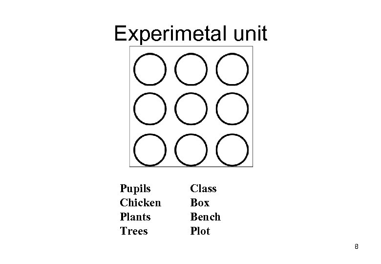Experimetal unit Pupils Chicken Plants Trees Class Box Bench Plot 8

3. “Mixed models”: Fixed and random factors Fixed factor: those who planned the experiment decided which levels to use Random factor: The levels are (or may be regarded as) a sample from a population of levels 9

Fixed and random factors Example: 40 forest stands. In each stand, one plot fertilized with A and one with B. Response variable: e. g. diameter of 5 trees on each plot Fixed factor: fertilizer, 2 levels (A and B) Experimental unit: the plot (NOT the tree!) Replication on 40 stands ”Stand” may be regarded as a random factor 10

Mixed models (cont. ) Examples of random factors • ”Block” in some designs • ”Individual”(when several measurements are made on each individual) • ”School class” (in experiments with teaching methods: then exp. unit is the class) • …i. e. in situations when many measurements are made on the same experimental unit. 11

Mixed models (cont. ) Mixed models are models that include both fixed and random factors. Programs for mixed models can also analyze models with only fixed, or only random, factors. 12

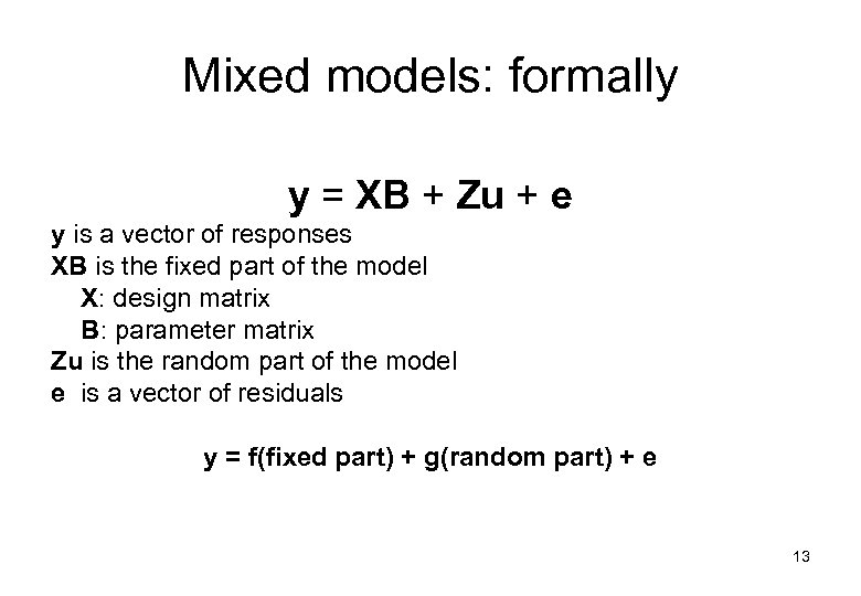Mixed models: formally y = XB + Zu + e y is a vector of responses XB is the fixed part of the model X: design matrix B: parameter matrix Zu is the random part of the model e is a vector of residuals y = f(fixed part) + g(random part) + e 13

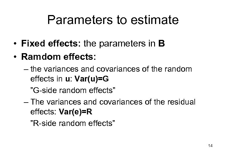Parameters to estimate • Fixed effects: the parameters in B • Ramdom effects: – the variances and covariances of the random effects in u: Var(u)=G ”G side random effects” – The variances and covariances of the residual effects: Var(e)=R ”R side random effects” 14

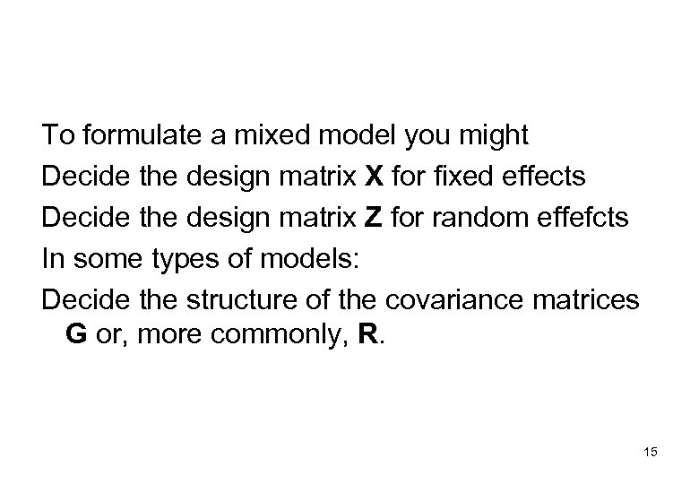To formulate a mixed model you might Decide the design matrix X for fixed effects Decide the design matrix Z for random effefcts In some types of models: Decide the structure of the covariance matrices G or, more commonly, R. 15

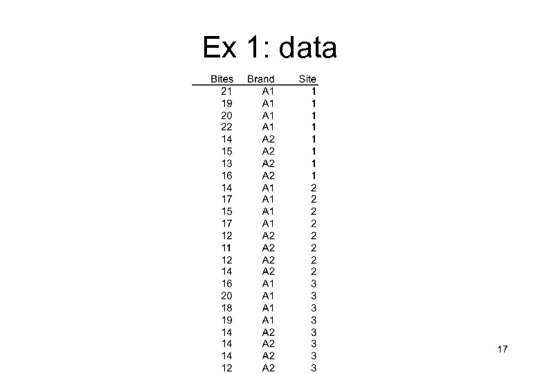
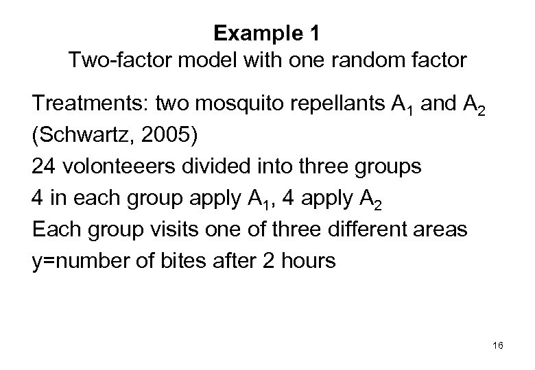Example 1 Two factor model with one random factor Treatments: two mosquito repellants A 1 and A 2 (Schwartz, 2005) 24 volonteeers divided into three groups 4 in each group apply A 1, 4 apply A 2 Each group visits one of three different areas y=number of bites after 2 hours 16

Ex 1: data 17

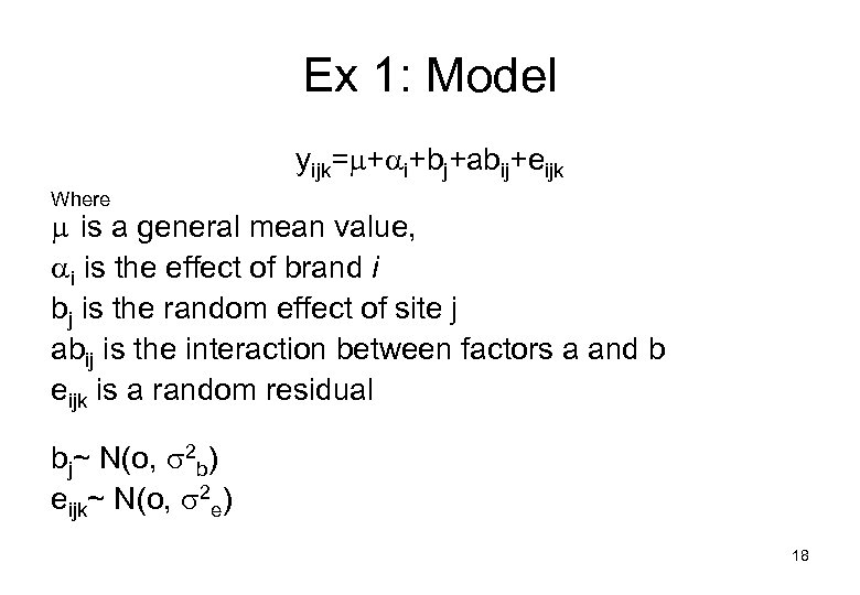Ex 1: Model yijk= + i+bj+abij+eijk Where is a general mean value, i is the effect of brand i bj is the random effect of site j abij is the interaction between factors a and b eijk is a random residual bj~ N(o, 2 b) eijk~ N(o, 2 e) 18

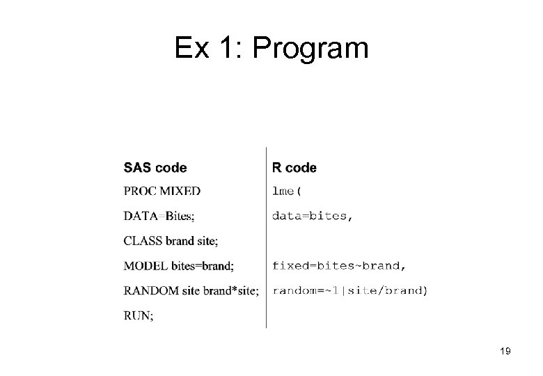Ex 1: Program 19

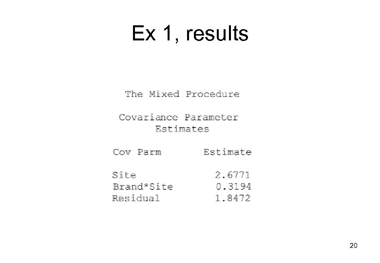Ex 1, results 20

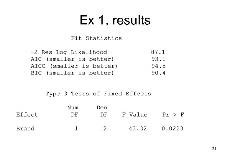Ex 1, results 21

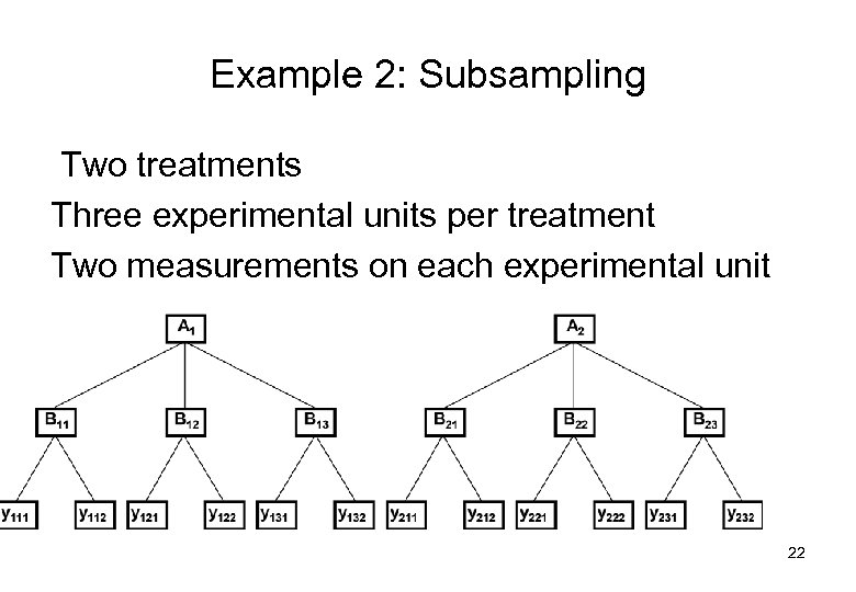Example 2: Subsampling Two treatments Three experimental units per treatment Two measurements on each experimental unit 22

Ex 2 An example of this type: 3 different fertilizers 4 plots with each fertilizer 2 mangold plants harvested from each plot y = iron content 23

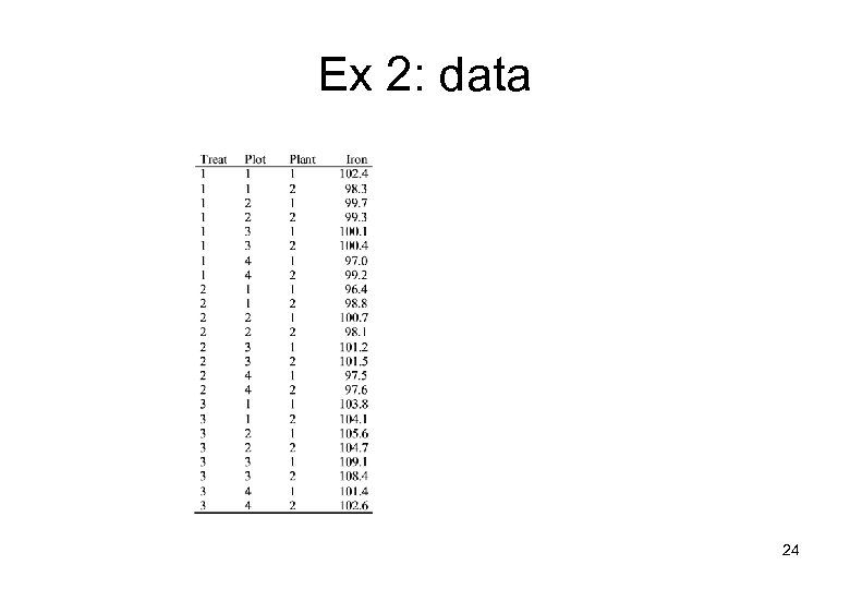Ex 2: data 24

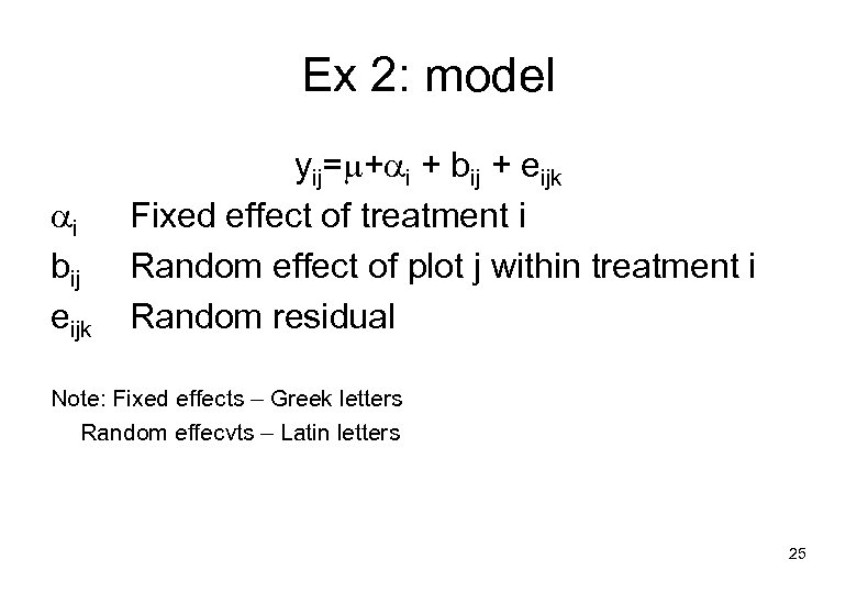Ex 2: model i bij eijk yij= + i + bij + eijk Fixed effect of treatment i Random effect of plot j within treatment i Random residual Note: Fixed effects – Greek letters Random effecvts – Latin letters 25

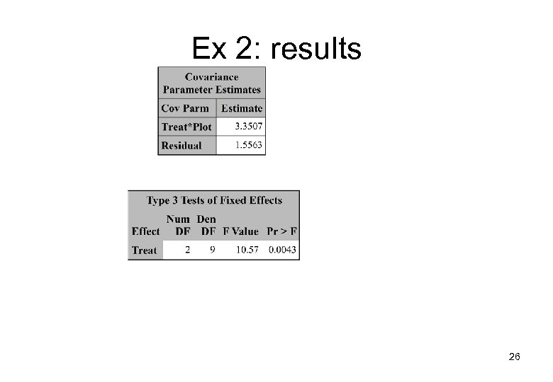Ex 2: results 26

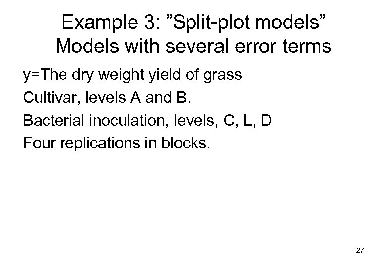Example 3: ”Split plot models” Models with several error terms y=The dry weight yield of grass Cultivar, levels A and B. Bacterial inoculation, levels, C, L, D Four replications in blocks. 27

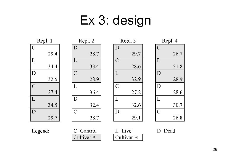Ex 3: design 28

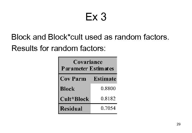Ex 3 Block and Block*cult used as random factors. Results for random factors: 29

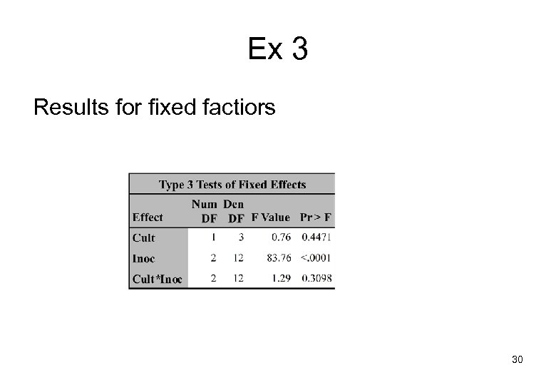Ex 3 Results for fixed factiors 30

Example 4: repeated measures 4 treatments 9 dogs per treatment Each dog measured at several time points 31

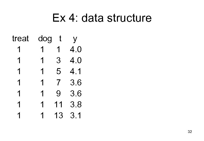Ex 4: data structure treat 1 1 1 1 dog t 1 1 1 3 1 5 1 7 1 9 1 11 1 13 y 4. 0 4. 1 3. 6 3. 8 3. 1 32

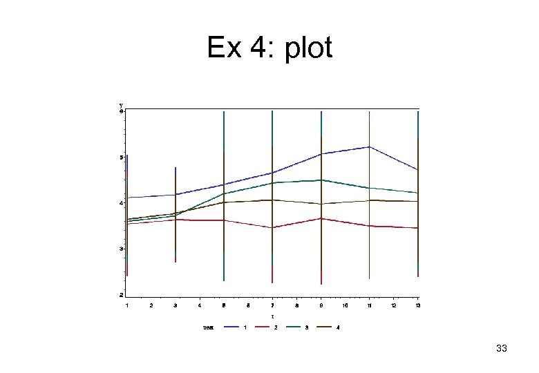Ex 4: plot 33

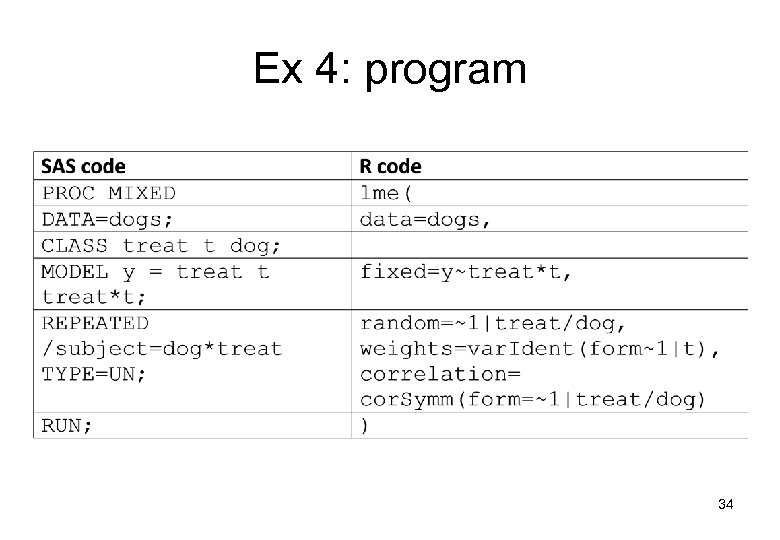Ex 4: program 34

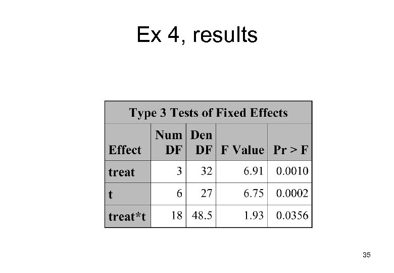Ex 4, results 35

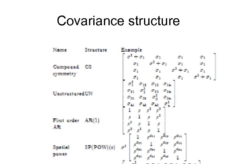
Covariance structures for repeated measurses data Model: y = XB + Zu + e The residuals e (”R side random effects”) are correlateded over time, correlation matrix R. If R is left free (unstructured) this gives tx(t 1)/2 parameters to estimate (t=# of time points). If n is small and t is large, we might run into peoblems (non vonvergence, negative definite Hessian matrix). 36

Covariance structure One solution: Apply some structure on R to reduce the number of parameters. 37

Covariance structure 38

Analysis strategy Baseline model: Time as a ”class” variable MODEL treatment time treatment*time; ”Repeated” part: First try UN. Simplify if needed: AR(1) for equidistant time points, else SP(POW) CS is only a last resort! To simplify the fixed part: Polynomials in time can be used. Or other known functions. 39

Other tricks Comparisons between models: Akaike’s Information Criterion (AIC) Denominator degrees of freedom for tests: Use the method by Kenward and Roger (1997) Normal distribution? Make diagnostic plots! Transformations? Robust (”sandwich”) estimators can be used or Generalized Linear Mixed Models… 40

Not covered… • Models with spatial variation – Lecture by Johannes Forkman • Models with non normal responses – (Generalized Linear Mixed Models) – Jan Eric’s talk; Computer session tromorrow • …and much more 41

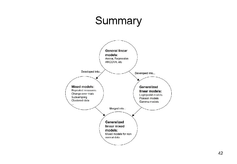Summary 42

”All models are wrong… …but some are useful. ” (G. E. P. Box) 43

References Fitzmaurice, G. M. , Laird, N. M. and Ware, J. H. (2004): Applied longitudinal analysis. New York, Wiley Littell, R. , Milliken, G. , Stroup, W. Wolfinger, R. and Schabenberger O. (2006): SAS for mixed models, second ed. Cary, N. C. , SAS Institute Inc. (R solutions to this can be found on the net) Ulf Olsson: Generalized linear models: an applied approach. Lund, Student litteratur, 2002 Ulf Olsson (2011): Statistics for Life Science 1. Lund, Studentlitteratur Ulf Olsson (2011): Statistics for Life Science 2. Lund, Studentlitteratur 44