Introduction to Knowledge Discovery and Data Mining Tu

Introduction to Knowledge Discovery and Data Mining Tu. Bao Ho (Hieu. Chi Dam) School of Knowledge Science Japan Advanced Institute of Science and Technology 19 November 2005

The lecture aims to … è Provide basic concepts and techniques of knowledge discovery and data mining (KDD). è Emphasize on different kinds of data, different tasks to do with the data, and different methods to do the tasks. è Emphasize on the KDD process and important issues when using data mining methods. 19 November 2005

Outline 1. Why knowledge discovery and data mining? 2. Basic concepts of KDD 3. KDD techniques: classification, association, clustering, text and Web mining 4. Challenges and trends in KDD 5. Case study in medicine data mining 19 November 2005

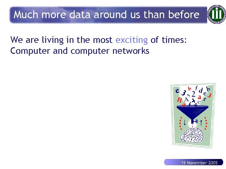Much more data around us than before We are living in the most exciting of times: Computer and computer networks 19 November 2005

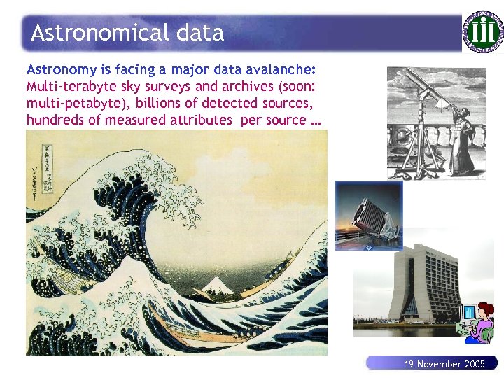Astronomical data Astronomy is facing a major data avalanche: Multi-terabyte sky surveys and archives (soon: multi-petabyte), billions of detected sources, hundreds of measured attributes per source … 19 November 2005

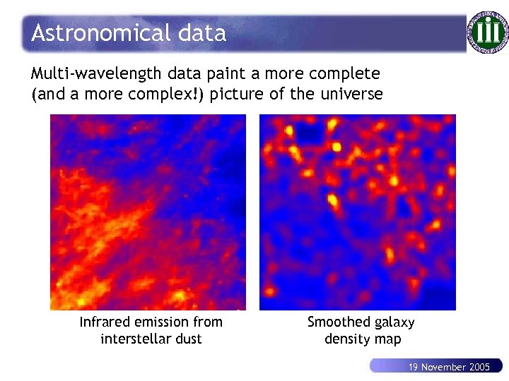Astronomical data Multi-wavelength data paint a more complete (and a more complex!) picture of the universe Infrared emission from interstellar dust Smoothed galaxy density map 19 November 2005

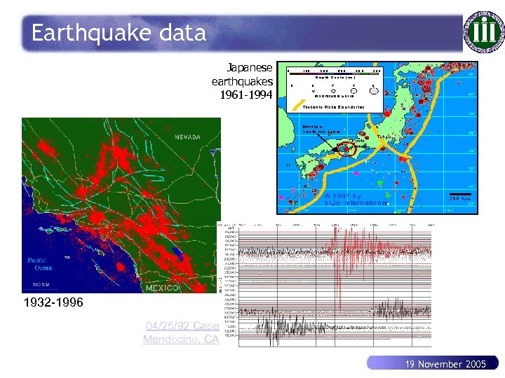Earthquake data Japanese earthquakes 1961 -1994 1932 -1996 04/25/92 Cape Mendocino, CA 19 November 2005

Predict earthquakes n 9 August 2004 (AP): Swedish geologists may have found a way to predict earthquakes weeks before they happen (current accurate warnings only come seconds before a quake). n Water samples taken 4, 900 feet beneath the ground in northern Iceland show the content of several metals increased dramatically a few weeks before a magnitude 5. 8 earthquake struck. n "We need a database over other earthquakes. " The bedrock at the test site is basalt, which is also found in other earthquake-prone areas like Hawaii and Japan. 19 November 2005

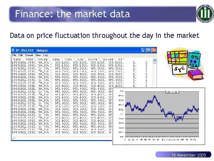Finance: the market data Data on price fluctuation throughout the day in the market 19 November 2005

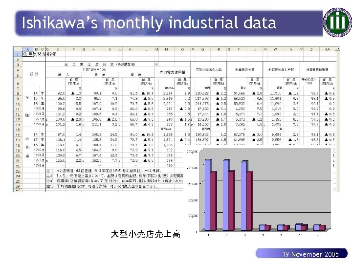Ishikawa’s monthly industrial data 大型小売店売上高 19 November 2005

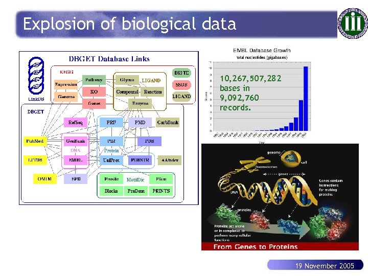Explosion of biological data 10, 267, 507, 282 bases in 9, 092, 760 records. 19 November 2005

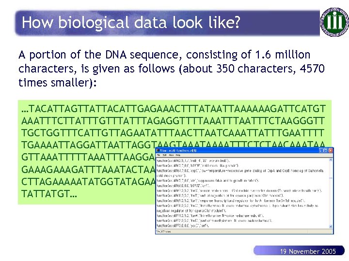How biological data look like? A portion of the DNA sequence, consisting of 1. 6 million characters, is given as follows (about 350 characters, 4570 times smaller): …TACATTAGTTATTACATTGAGAAACTTTATAATTAAAAAAGATTCATGT AAATTTCTTATTTGTTTAGAGGTTTTAAATTTCTAAGGGTT TGCTGGTTTCATTGTTAGAATATTTAACTTAATCAAATTATTTGAATTTT TGAAAATTAGGATTAGGTAAATAAAATTTCTCTAACAAATAA GTTAAATTTAAGGAGATAAAAATACTACTCTGTTTTATTATG GAAAGATTTAAATACTAAAGGGTTTATATGAAGTAGTTACC CTTAGAAAAATATGGTATAGAAAGCTTAAATATTAAGAGTGATGAAGTA TATTATGT… 19 November 2005

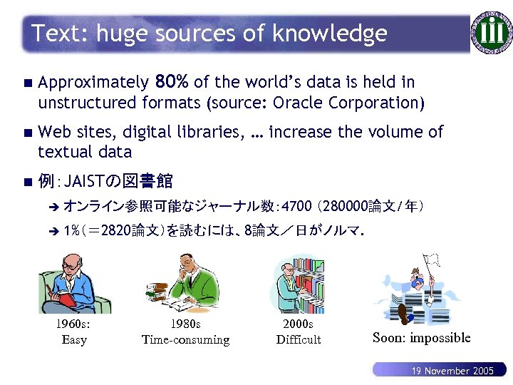Text: huge sources of knowledge n Approximately 80% of the world’s data is held in unstructured formats (source: Oracle Corporation) n Web sites, digital libraries, … increase the volume of textual data n 例：JAISTの図書館 è オンライン参照可能なジャーナル数： 4700 （280000論文/年） è 1%（＝ 2820論文）を読むには、8論文／日がノルマ. 1960 s: Easy 1980 s Time-consuming 2000 s Difficult Soon: impossible 19 November 2005

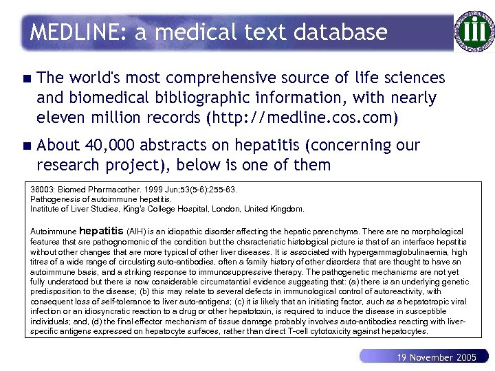MEDLINE: a medical text database n The world's most comprehensive source of life sciences and biomedical bibliographic information, with nearly eleven million records (http: //medline. cos. com) n About 40, 000 abstracts on hepatitis (concerning our research project), below is one of them 36003: Biomed Pharmacother. 1999 Jun; 53(5 -6): 255 -63. Pathogenesis of autoimmune hepatitis. Institute of Liver Studies, King's College Hospital, London, United Kingdom. Autoimmune hepatitis (AIH) is an idiopathic disorder affecting the hepatic parenchyma. There are no morphological features that are pathognomonic of the condition but the characteristic histological picture is that of an interface hepatitis without other changes that are more typical of other liver diseases. It is associated with hypergammaglobulinaemia, high titres of a wide range of circulating auto-antibodies, often a family history of other disorders that are thought to have an autoimmune basis, and a striking response to immunosuppressive therapy. The pathogenetic mechanisms are not yet fully understood but there is now considerable circumstantial evidence suggesting that: (a) there is an underlying genetic predisposition to the disease; (b) this may relate to several defects in immunological control of autoreactivity, with consequent loss of self-tolerance to liver auto-antigens; (c) it is likely that an initiating factor, such as a hepatotropic viral infection or an idiosyncratic reaction to a drug or other hepatotoxin, is required to induce the disease in susceptible individuals; and, (d) the final effector mechanism of tissue damage probably involves auto-antibodies reacting with liverspecific antigens expressed on hepatocyte surfaces, rather than direct T-cell cytotoxicity against hepatocytes. 19 November 2005

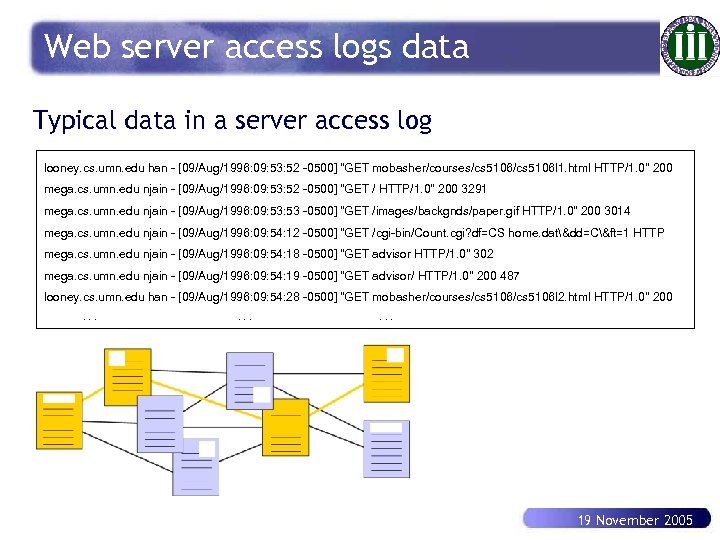Web server access logs data Typical data in a server access log looney. cs. umn. edu han - [09/Aug/1996: 09: 53: 52 -0500] "GET mobasher/courses/cs 5106 l 1. html HTTP/1. 0" 200 mega. cs. umn. edu njain - [09/Aug/1996: 09: 53: 52 -0500] "GET / HTTP/1. 0" 200 3291 mega. cs. umn. edu njain - [09/Aug/1996: 09: 53 -0500] "GET /images/backgnds/paper. gif HTTP/1. 0" 200 3014 mega. cs. umn. edu njain - [09/Aug/1996: 09: 54: 12 -0500] "GET /cgi-bin/Count. cgi? df=CS home. dat&dd=C&ft=1 HTTP mega. cs. umn. edu njain - [09/Aug/1996: 09: 54: 18 -0500] "GET advisor HTTP/1. 0" 302 mega. cs. umn. edu njain - [09/Aug/1996: 09: 54: 19 -0500] "GET advisor/ HTTP/1. 0" 200 487 looney. cs. umn. edu han - [09/Aug/1996: 09: 54: 28 -0500] "GET mobasher/courses/cs 5106 l 2. html HTTP/1. 0" 200. . 19 November 2005

Web link data Internet Map [lumeta. com] Friendship Network [Moody ’ 01] Food Web [Martinez ’ 91] 19 November 2005

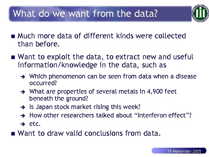What do we want from the data? n Much more data of different kinds were collected than before. n Want to exploit the data, to extract new and useful information/knowledge in the data, such as è è è n Which phenomenon can be seen from data when a disease occurred? What are properties of several metals in 4, 900 feet beneath the ground? Is Japan stock market rising this week? How other researchers talked about “interferon effect”? etc. Want to draw valid conclusions from data. 19 November 2005

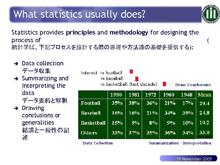What statistics usually does? Statistics provides principles and methodology for designing the process of ( 統計学は、下記プロセスを設計する際の原理や方法論の基礎を提供する): è è è Data collection データ収集 Summarizing and Interpreting the data データ要約と解釈 Drawing conclusions or generalities 結論と一般性の記 述 19 November 2005

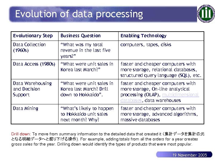Evolution of data processing Evolutionary Step Business Question Enabling Technology Data Collection (1960 s) “What was my total revenue in the last five years? ” computers, tapes, disks Data Access (1980 s) “What were unit sales in Korea last March? ” faster and cheaper computers with more storage, relational databases, structured query language (SQL), etc. Data Warehousing and Decision Support “What were unit sales in Korea last March? Drill down to Hokkaido”. faster and cheaper computers with more storage, On-line analytical processing (OLAP), multidimensional databases, data warehouses Data Mining “What’s likely to happen to Hokkaido unit sales next month? Why? faster and cheaper computers with more storage, advanced algorithms, massive databases Drill down: To move from summary information to the detailed data that created it （集計データを集計の元 となる明細データへと掘り下げる操作). For example, adding totals from all the orders for a year creates gross sales for the year. Drilling down would identify the types of products that were most popular. 19 November 2005

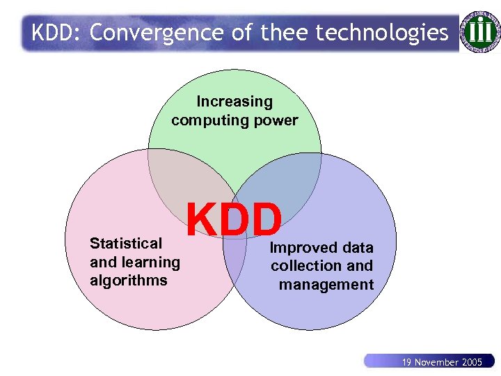KDD: Convergence of thee technologies Increasing computing power Statistical and learning algorithms KDD Improved data collection and management 19 November 2005

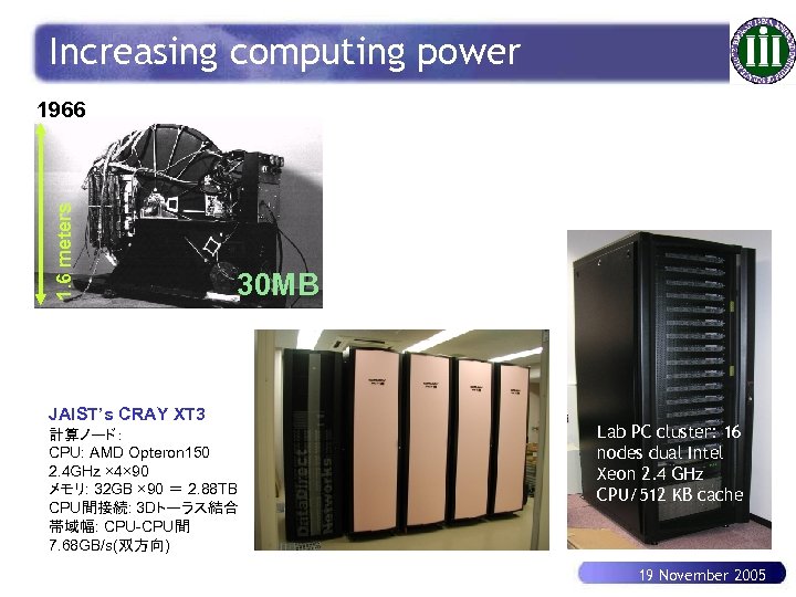Increasing computing power 1. 6 meters 1966 30 MB JAIST’s CRAY XT 3 計算ノード： 　　 CPU: AMD Opteron 150 2. 4 GHz × 4× 90 　　 メモリ: 32 GB × 90 ＝ 2. 88 TB 　　 CPU間接続: 3 Dトーラス結合 　　 帯域幅: CPU-CPU間　 7. 68 GB/s(双方向) Lab PC cluster: 16 nodes dual Intel Xeon 2. 4 GHz CPU/512 KB cache 19 November 2005

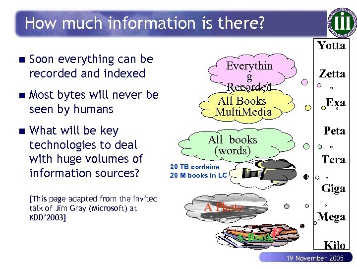How much information is there? Yotta n Soon everything can be recorded and indexed n Most bytes will never be seen by humans n What will be key technologies to deal with huge volumes of information sources? Everythin g Recorded All Books Multi. Media Tera. Movie [This page adapted from the invited talk of Jim Gray (Microsoft) at KDD’ 2003] Exa Peta All books (words) 20 TB contains 20 M books in LC Zetta A Photo A Book Giga Mega Kilo 19 November 2005

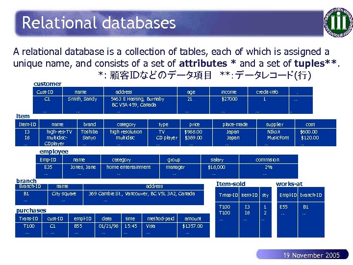Relational databases A relational database is a collection of tables, each of which is assigned a unique name, and consists of a set of attributes * and a set of tuples**. 　　　　　　　*: 顧客IDなどのデータ項目　**：データレコード(行) customer Cust-ID C 1 name Smith, Sandy … item Item-ID I 3 I 8 … … name high-res-TV multidisc. CDplayer brand Toshiba Sanyo … address 5463 E Hasting, Burnaby BC V 5 A 459, Canada … age 21 … category high resolution multidisc … price $988. 00 $369. 00 … type TV CD player … income $27000 credit-info 1 … … place-made Japan … . … … supplier NIko. X Music. Font … cost $600. 00 $120. 00 … employee Emp-ID E 35 … branch Branch-ID B 1 … name Jones, Jane … name City square … category home entertainment … group manager … address 369 Cambie St. , Vancouver, BC V 5 L 3 A 2, Canada … purchases Trans-ID T 100 … cust-ID C 1. … empl-ID B 55 … data 01/21/98 … time 15: 45 … method-paid Visa … amount $1357. 00 … salary $18, 000 … commision 2% … Item-sold works-at Trnas-ID item-ID sty Empl-ID branch-ID T 100 … E 55 … I 3 I 8 … 1 2 … B 1 … 19 November 2005

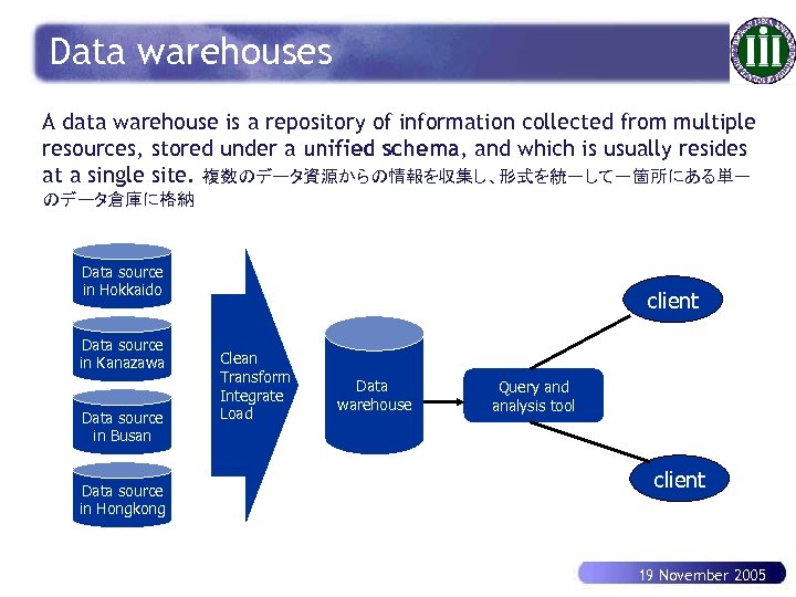Data warehouses A data warehouse is a repository of information collected from multiple resources, stored under a unified schema, and which is usually resides at a single site. 複数のデータ資源からの情報を収集し、形式を統一して一箇所にある単一 のデータ倉庫に格納 Data source in Hokkaido Data source in Kanazawa Data source in Busan Data source in Hongkong client Clean Transform Integrate Load Data warehouse Query and analysis tool client 19 November 2005

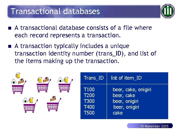Transactional databases n A transactional database consists of a file where each record represents a transaction. n A transaction typically includes a unique transaction identity number (trans_ID), and list of the items making up the transaction. Trans_ID T 100 T 200 T 300 T 400 T 500 list of item_ID beer, cake, onigiri beer, cake beer, onigiri cake 19 November 2005

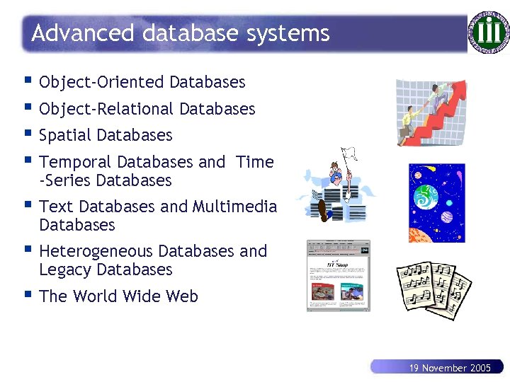Advanced database systems § Object-Oriented Databases § Object-Relational Databases § Spatial Databases § Temporal Databases and Time -Series Databases § Text Databases and Multimedia Databases § Heterogeneous Databases and Legacy Databases § The World Wide Web 19 November 2005

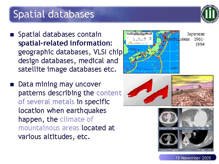Spatial databases n Spatial databases contain spatial-related information: geographic databases, VLSI chip design databases, medical and satellite image databases etc. n Data mining may uncover patterns describing the content of several metals in specific location when earthquakes happen, the climate of mountainous areas located at various altitudes, etc. Japanese earthquakes 19611994 19 November 2005

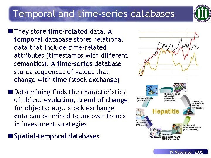Temporal and time-series databases n They store time-related data. A temporal database stores relational data that include time-related attributes (timestamps with different semantics). A time-series database stores sequences of values that change with time (stock exchange) n Data mining finds the characteristics of object evolution, trend of change for objects: e. g. , stock exchange data can be mined to uncover trends in investment strategies n Spatial-temporal databases 19 November 2005

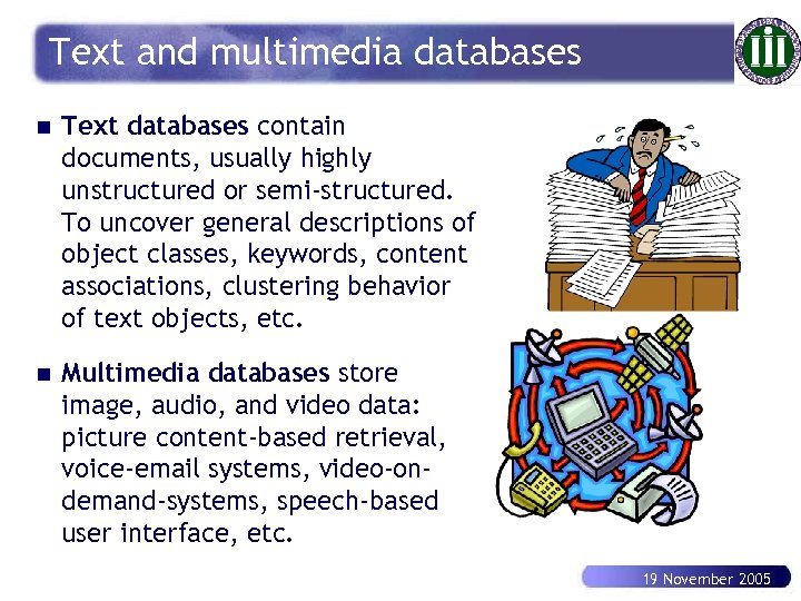Text and multimedia databases n Text databases contain documents, usually highly unstructured or semi-structured. To uncover general descriptions of object classes, keywords, content associations, clustering behavior of text objects, etc. n Multimedia databases store image, audio, and video data: picture content-based retrieval, voice-email systems, video-ondemand-systems, speech-based user interface, etc. 19 November 2005

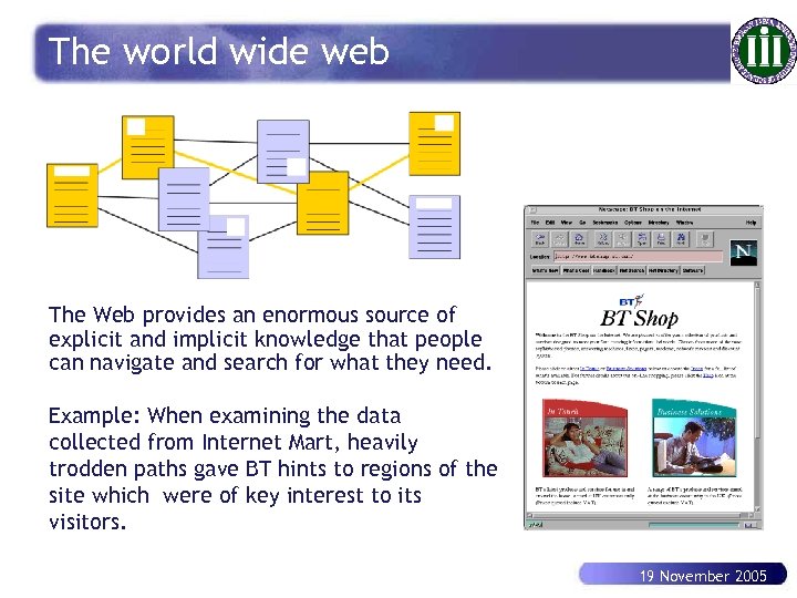The world wide web The Web provides an enormous source of explicit and implicit knowledge that people can navigate and search for what they need. Example: When examining the data collected from Internet Mart, heavily trodden paths gave BT hints to regions of the site which were of key interest to its visitors. 19 November 2005

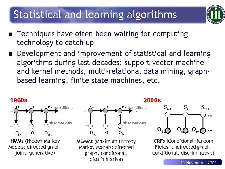Statistical and learning algorithms n n Techniques have often been waiting for computing technology to catch up Development and improvement of statistical and learning algorithms during last decades: support vector machine and kernel methods, multi-relational data mining, graphbased learning, finite state machines, etc. 1960 s. . . t-1 2000 s t t+1 transitions . . . observations . . . Ot -1 Ot . . . t-1 t . . . Ot+1 HMMs (Hidden Markov Models: directed graph, joint, generative) t+1 transitions . . . St-1 St St+1. . . observations Ot -1 Ot Ot+1 MEMMs (Maximum Entropy Markov Models: directed graph, conditional, discriminative) Ot-1 Ot Ot+1 . . . CRFs (Conditional Random Fields: undirected graph, conditional, discriminative) 19 November 2005

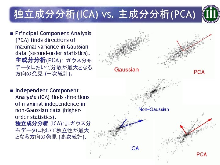独立成分分析(ICA) vs. 主成分分析(PCA) n Principal Component Analysis (PCA) finds directions of maximal variance in Gaussian data (second-order statistics). 主成分分析(PCA)： ガウス分布 データにおいて分散が最大となる 方向の発見 (一次統計). n Independent Component Analysis (ICA) finds directions of maximal independence in non-Gaussian data (higherorder statistics). 独立成分分析 (ICA)：非ガウス分 布データにおいて独立性が最大 となる方向の発見 (高次統計). 19 November 2005

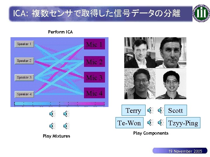ICA: 複数センサで取得した信号データの分離 Perform ICA Mic 1 Mic 2 Mic 3 Mic 4 Terry Te-Won Play Mixtures Scott Tzyy-Ping Play Components 19 November 2005

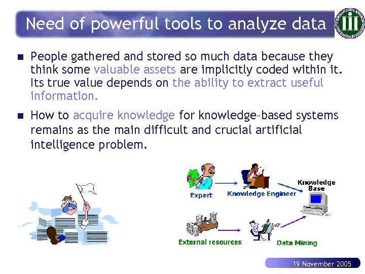Need of powerful tools to analyze data n People gathered and stored so much data because they think some valuable assets are implicitly coded within it. Its true value depends on the ability to extract useful information. n How to acquire knowledge for knowledge–based systems remains as the main difficult and crucial artificial intelligence problem. 19 November 2005

Outline 1. Why knowledge discovery and data mining? 2. Basic concepts of KDD 3. KDD techniques: classification, association, clustering, text and Web mining 4. Challenges and trends in KDD 5. Case study in medicine data mining 19 November 2005

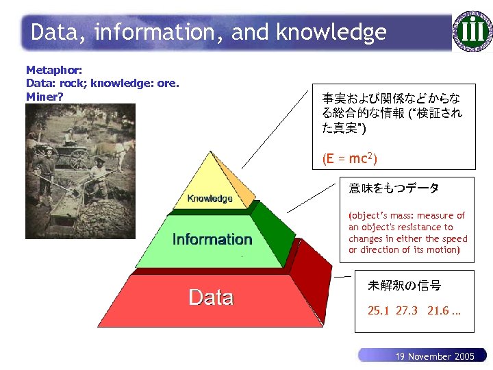Data, information, and knowledge Metaphor: Data: rock; knowledge: ore. Miner? 事実および関係などからな る総合的な情報 (“検証され た真実”) (E = mc 2) 意味をもつデータ (object’s mass: measure of an object's resistance to changes in either the speed or direction of its motion) 未解釈の信号 25. 1 27. 3 21. 6 … 19 November 2005

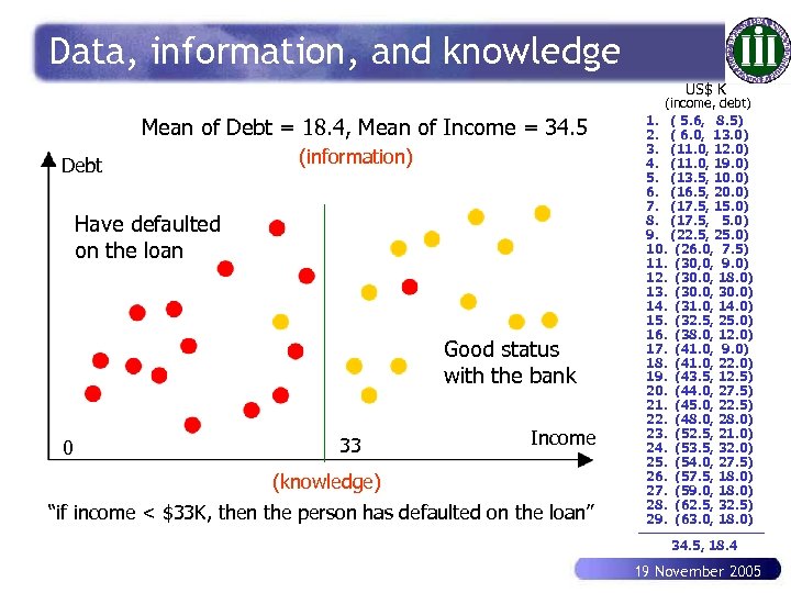Data, information, and knowledge US$ K Mean of Debt = 18. 4, Mean of Income = 34. 5 Debt (information) Have defaulted on the loan Good status with the bank 0 33 Income (knowledge) “if income < $33 K, then the person has defaulted on the loan” (income, debt) 1. ( 5. 6, 8. 5) 2. ( 6. 0, 13. 0) 3. (11. 0, 12. 0) 4. (11. 0, 19. 0) 5. (13. 5, 10. 0) 6. (16. 5, 20. 0) 7. (17. 5, 15. 0) 8. (17. 5, 5. 0) 9. (22. 5, 25. 0) 10. (26. 0, 7. 5) 11. (30, 0, 9. 0) 12. (30. 0, 18. 0) 13. (30. 0, 30. 0) 14. (31. 0, 14. 0) 15. (32. 5, 25. 0) 16. (38. 0, 12. 0) 17. (41. 0, 9. 0) 18. (41. 0, 22. 0) 19. (43. 5, 12. 5) 20. (44. 0, 27. 5) 21. (45. 0, 22. 5) 22. (48. 0, 28. 0) 23. (52. 5, 21. 0) 24. (53. 5, 32. 0) 25. (54. 0, 27. 5) 26. (57. 5, 18. 0) 27. (59. 0, 18. 0) 28. (62. 5, 32. 5) 29. (63. 0, 18. 0) 34. 5, 18. 4 19 November 2005

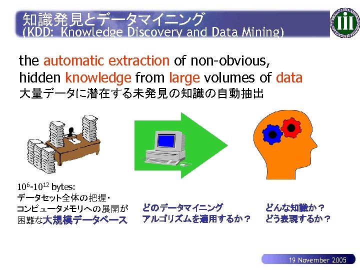知識発見とデータマイニング (KDD: Knowledge Discovery and Data Mining) the automatic extraction of non-obvious, hidden knowledge from large volumes of data 大量データに潜在する未発見の知識の自動抽出 106 -1012 bytes: データセット全体の把握・ コンピュータメモリへの展開が 困難な大規模データベース どのデータマイニング アルゴリズムを適用するか？ どんな知識か？ どう表現するか？ 19 November 2005

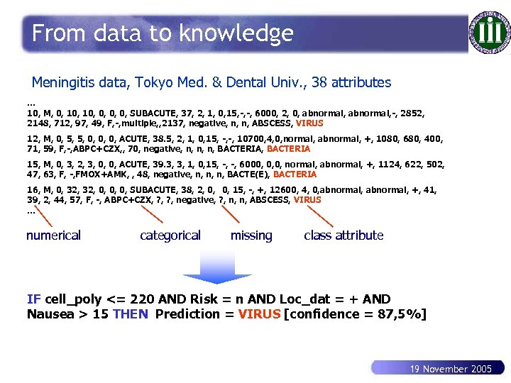From data to knowledge Meningitis data, Tokyo Med. & Dental Univ. , 38 attributes. . . 10, M, 0, 10, 0, SUBACUTE, 37, 2, 1, 0, 15, -, -, 6000, 2, 0, abnormal, -, 2852, 2148, 712, 97, 49, F, -, multiple, , 2137, negative, n, n, ABSCESS, VIRUS 12, M, 0, 5, 5, 0, 0, 0, ACUTE, 38. 5, 2, 1, 0, 15, -, -, 10700, 4, 0, normal, abnormal, +, 1080, 680, 400, 71, 59, F, -, ABPC+CZX, , 70, negative, n, n, n, BACTERIA 15, M, 0, 3, 2, 3, 0, 0, ACUTE, 39. 3, 3, 1, 0, 15, -, -, 6000, 0, 0, normal, abnormal, +, 1124, 622, 502, 47, 63, F, -, FMOX+AMK, , 48, negative, n, n, n, BACTE(E), BACTERIA 16, M, 0, 32, 0, 0, 0, SUBACUTE, 38, 2, 0, 　 15, -, +, 12600, 4, 0, abnormal, +, 41, 0, 39, 2, 44, 57, F, -, ABPC+CZX, ? , negative, ? , n, n, ABSCESS, VIRUS. . . numerical categorical missing class attribute IF cell_poly <= 220 AND Risk = n AND Loc_dat = + AND Nausea > 15 THEN Prediction = VIRUS [confidence = 87, 5%] 19 November 2005

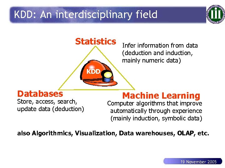KDD: An interdisciplinary field Statistics Infer information from data (deduction and induction, mainly numeric data) KDD Databases Store, access, search, update data (deduction) Machine Learning Computer algorithms that improve automatically through experience (mainly induction, symbolic data) also Algorithmics, Visualization, Data warehouses, OLAP, etc. 19 November 2005

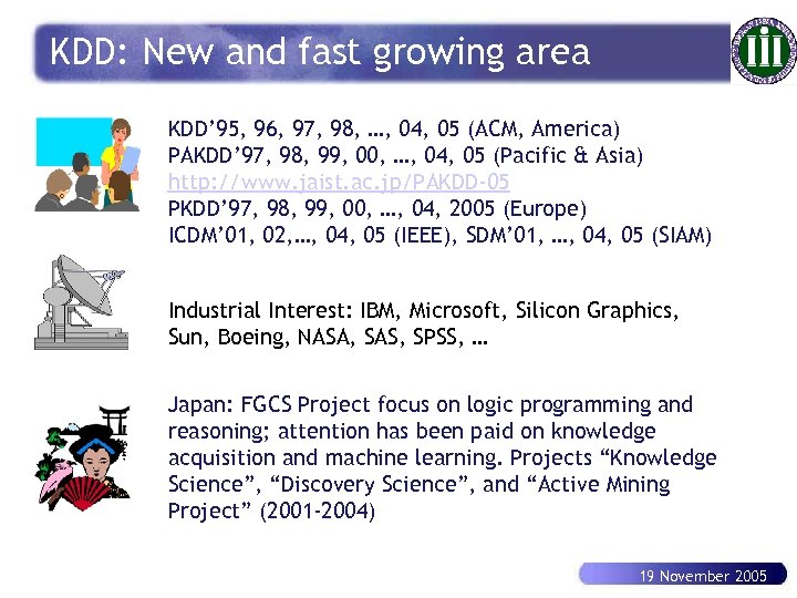KDD: New and fast growing area KDD’ 95, 96, 97, 98, …, 04, 05 (ACM, America) PAKDD’ 97, 98, 99, 00, …, 04, 05 (Pacific & Asia) http: //www. jaist. ac. jp/PAKDD-05 PKDD’ 97, 98, 99, 00, …, 04, 2005 (Europe) ICDM’ 01, 02, …, 04, 05 (IEEE), SDM’ 01, …, 04, 05 (SIAM) Industrial Interest: IBM, Microsoft, Silicon Graphics, Sun, Boeing, NASA, SAS, SPSS, … Japan: FGCS Project focus on logic programming and reasoning; attention has been paid on knowledge acquisition and machine learning. Projects “Knowledge Science”, “Discovery Science”, and “Active Mining Project” (2001 -2004) 19 November 2005

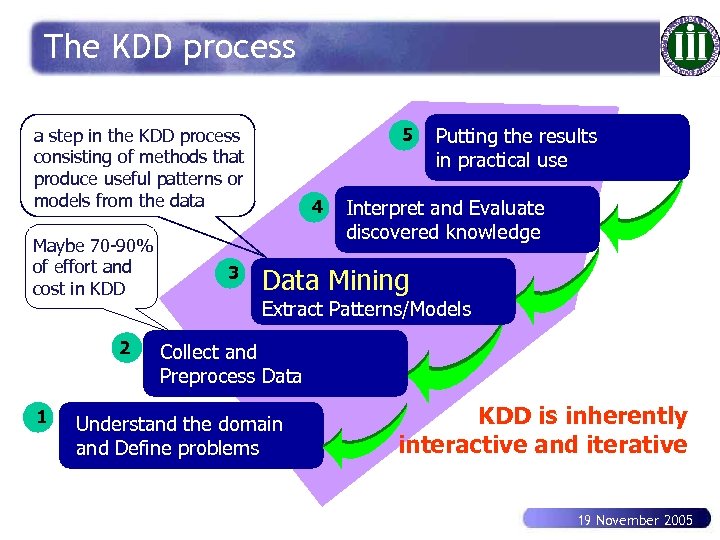The KDD process 5 a step in the KDD process consisting of methods that produce useful patterns or models from the data Maybe 70 -90% of effort and cost in KDD 2 1 3 4 Putting the results in practical use Interpret and Evaluate discovered knowledge Data Mining Extract Patterns/Models Collect and Preprocess Data Understand the domain and Define problems KDD is inherently interactive and iterative 19 November 2005

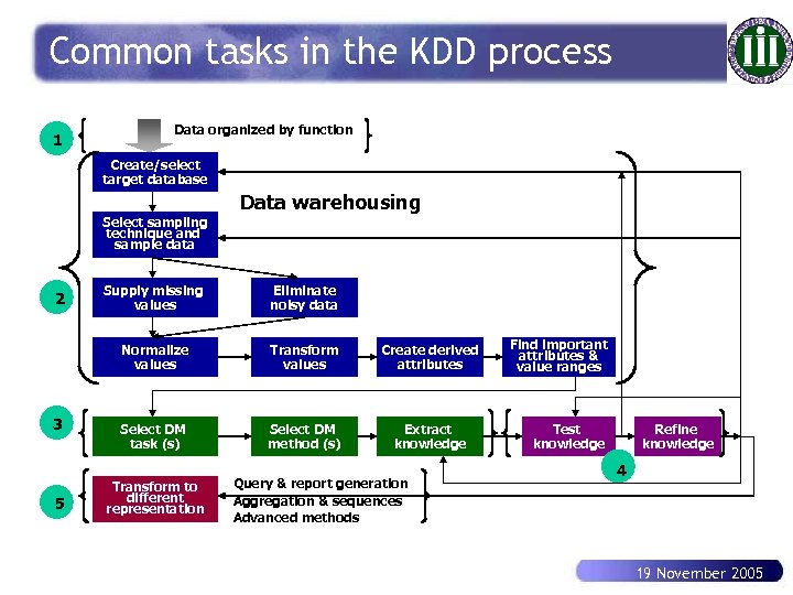Common tasks in the KDD process 1 Data organized by function Create/select target database Data warehousing Select sampling technique and sample data 3 5 Supply missing values Eliminate noisy data Normalize values 2 Transform values Create derived attributes Select DM task (s) Select DM method (s) Extract knowledge Transform to different representation Query & report generation Aggregation & sequences Advanced methods Find important attributes & value ranges Test knowledge Refine knowledge 4 19 November 2005

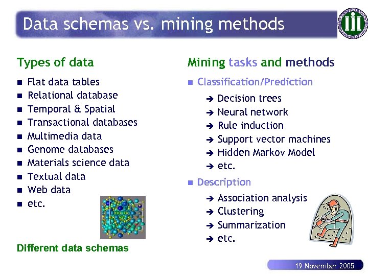Data schemas vs. mining methods Types of data n n n n n Flat data tables Relational database Temporal & Spatial Transactional databases Multimedia data Genome databases Materials science data Textual data Web data etc. Different data schemas Mining tasks and methods n Classification/Prediction Decision trees è Neural network è Rule induction è Support vector machines è Hidden Markov Model è etc. è n Description Association analysis è Clustering è Summarization è etc. è 19 November 2005

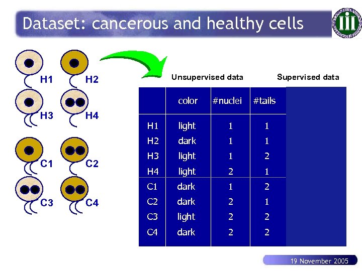Dataset: cancerous and healthy cells H 1 Unsupervised data H 2 color H 3 H 4 #nuclei Supervised data #tails class C 3 C 4 1 1 healthy dark 1 1 healthy H 3 light 1 2 healthy H 4 light 2 1 healthy C 1 C 2 light H 2 C 1 H 1 dark 1 2 cancerous C 2 dark 2 1 cancerous C 3 light 2 2 cancerous C 4 dark 2 2 cancerous 19 November 2005

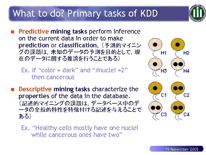What to do? Primary tasks of KDD n Predictive mining tasks perform inference on the current data in order to make prediction or classification. （予測的マイニン グの課題は，未知のデータの予測を目的として，現 在のデータに関する推論を行うことである） Ex. If “color = dark” and “#nuclei =2” then cancerous n Descriptive mining tasks characterize the properties of the data in the database. （記述的マイニングの課題は，データベース中のデ ータの全般的特性を特徴付ける記述を与えることで ある） Ex. “Healthy cells mostly have one nuclei while cancerous ones have two” 19 November 2005

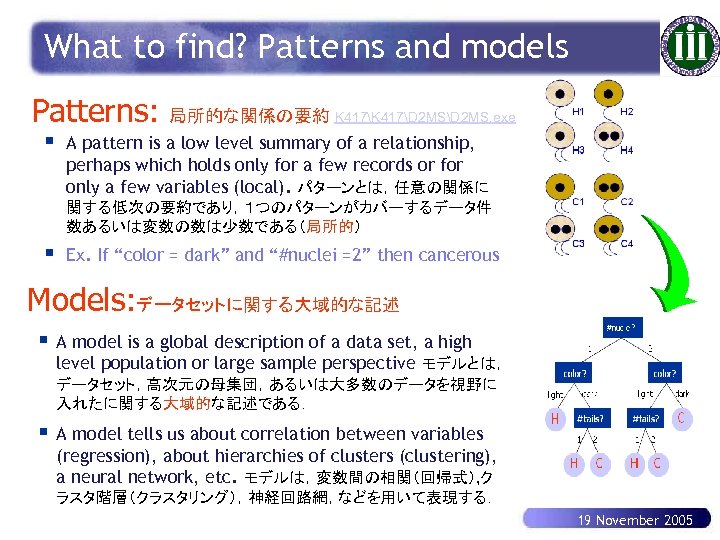What to find? Patterns and models Patterns: § 局所的な関係の要約 K 417D 2 MSD 2 MS. exe A pattern is a low level summary of a relationship, perhaps which holds only for a few records or for only a few variables (local). パターンとは，任意の関係に 関する低次の要約であり，１つのパターンがカバーするデータ件 数あるいは変数の数は少数である（局所的）　 § Ex. If “color = dark” and “#nuclei =2” then cancerous Models: データセットに関する大域的な記述 § A model is a global description of a data set, a high level population or large sample perspective モデルとは， データセット，高次元の母集団，あるいは大多数のデータを視野に 入れたに関する大域的な記述である． § A model tells us about correlation between variables (regression), about hierarchies of clusters (clustering), a neural network, etc. モデルは，変数間の相関（回帰式）, ク ラスタ階層（クラスタリング），神経回路網，などを用いて表現する． 19 November 2005

Classification/Prediction Classification/prediction is the process of finding a set of models (or patterns) that describe and distinguish data classes or concepts, for the purpose of being able to use the model to predict the class of objects whose class label is unknown （分類*/予測**とは，データのクラス/概念を説明し識別する一連のモデルを 見つけ出すプロセスであり，このモデルを用い，クラス情報が不明なデータの 分類を予測する　*カテゴリデータの場合　**数値データの場合） è è è Decision trees IF-THEN rules Neural networks Support vector machines etc. 19 November 2005

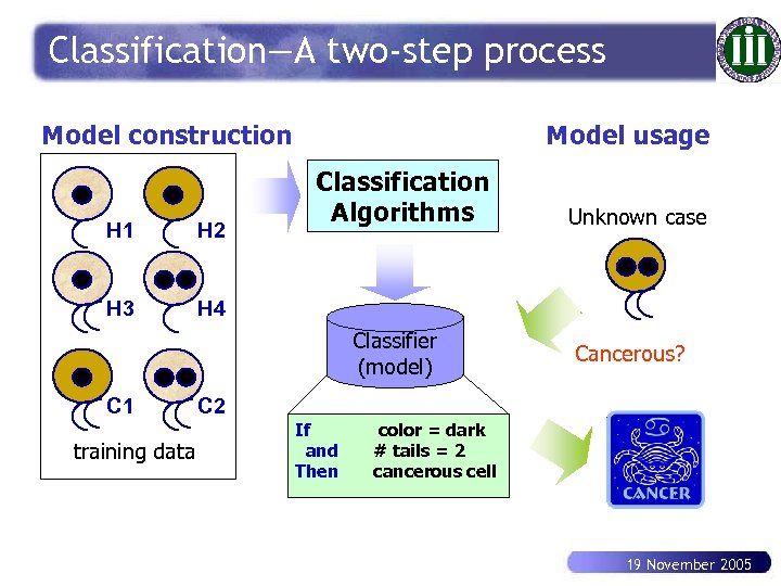Classification—A two-step process Model construction H 1 H 2 H 3 Model usage Classification Algorithms Unknown case H 4 Classifier (model) C 1 training data Cancerous? C 2 If and Then color = dark # tails = 2 cancerous cell 19 November 2005

Criteria for classification methods n Predictive accuracy（予測精度）: the ability of the classifier to correctly predict unseen data n Speed: refers to computation cost n Robustness（頑健性）: the ability of the classifier to make correctly predictions given noisy data or data with missing values n Scalability（拡張性）: the ability to construct the classifier efficiently given large amounts of data n Interpretability（解釈容易性）: the level of understanding and insight that is provided by the classifier 19 November 2005

Description is the process of finding a set of patterns or models that describe properties of data (essentially the summary of data), for the purpose of understanding the data. （記述とは、データの理解を目的とし、そのデータを要約するような性質を表 現するパターンあるいはモデル集合を発見する過程である） è è è Clustering Association mining Summarization Trend detection etc. 19 November 2005

Criteria for description methods n Interestingness: overall measure combining novelty, utility, simplicity, reliability and validity of discovered patterns/models. n Speed: refers to computation cost n Scalability（拡張性）: the ability to construct the classifier efficiently given large amounts of data n Interpretability（解釈容易性）: the level of understanding and insight that is provided by the classifier 19 November 2005

Outline 1. Why knowledge discovery and data mining? 2. Basic concepts of KDD 3. KDD techniques: classification, association, clustering, text and Web mining 4. Challenges and trends in KDD 5. Case study in medicine data mining 19 November 2005

Decision tree learning Learn to generate classifiers in the form of decision trees from supervised data. 19 November 2005

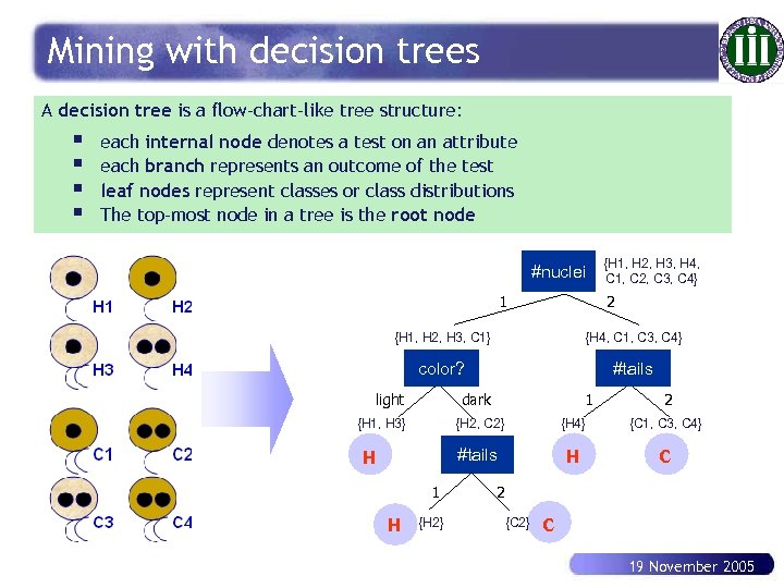Mining with decision trees A decision tree is a flow-chart-like tree structure: § § each internal node denotes a test on an attribute each branch represents an outcome of the test leaf nodes represent classes or class distributions The top-most node in a tree is the root node #nuclei 1 {H 1, H 2, H 3, H 4, C 1, C 2, C 3, C 4} 2 {H 1, H 2, H 3, C 1} {H 4, C 1, C 3, C 4} color? #tails light dark {H 1, H 3} 1 2 {H 2, C 2} 1 H {H 2} {C 1, C 3, C 4} #tails H {H 4} H C 2 {C 2} C 19 November 2005

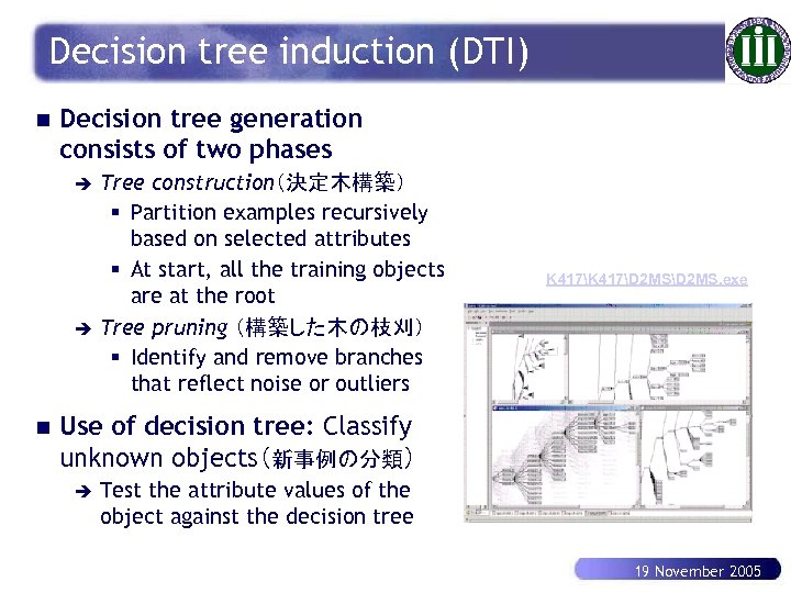Decision tree induction (DTI) n Decision tree generation consists of two phases è è n Tree construction（決定木構築） § Partition examples recursively based on selected attributes § At start, all the training objects are at the root Tree pruning （構築した木の枝刈） § Identify and remove branches that reflect noise or outliers K 417D 2 MSD 2 MS. exe Use of decision tree: Classify unknown objects（新事例の分類） è Test the attribute values of the object against the decision tree 19 November 2005

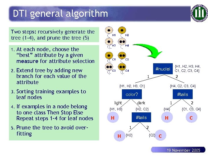DTI general algorithm Two steps: recursively generate the tree (1 -4), and prune the tree (5) 1. 2. At each node, choose the “best” attribute by a given measure for attribute selection Extend tree by adding new branch for each value of the attribute 3. Sorting training examples to leaf nodes 4. If examples in a node belong to one class Then Stop Else Repeat steps 1 -4 for leaf nodes 5. #nuclei Prune the tree to avoid overfitting 1 {H 1, H 2, H 3, H 4, C 1, C 2, C 3, C 4} 2 {H 1, H 2, H 3, C 1} {H 4, C 2, C 3, C 4} color? #tails light dark {H 1, H 3} 1 2 {H 2, C 2} 1 H {H 2} {C 1, C 3, C 4} #tails H {H 4} H C 2 {C 2} C 19 November 2005

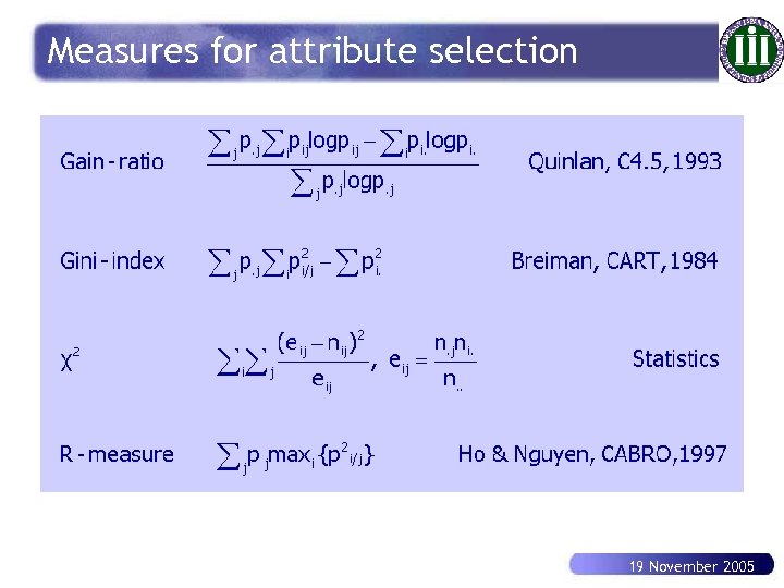Measures for attribute selection 19 November 2005

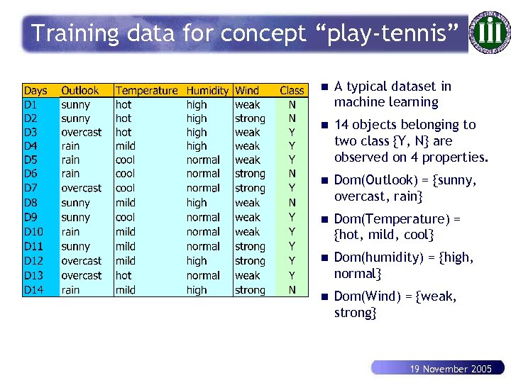Training data for concept “play-tennis” n A typical dataset in machine learning n 14 objects belonging to two class {Y, N} are observed on 4 properties. n Dom(Outlook) = {sunny, overcast, rain} n Dom(Temperature) = {hot, mild, cool} n Dom(humidity) = {high, normal} n Dom(Wind) = {weak, strong} 19 November 2005

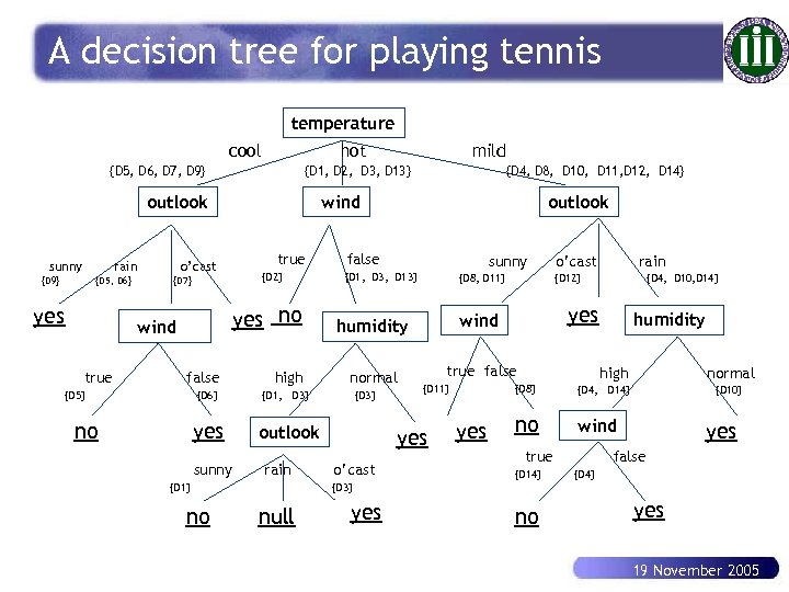A decision tree for playing tennis temperature cool hot {D 5, D 6, D 7, D 9} {D 1, D 2, D 3, D 13} outlook sunny rain {D 9} {D 5, D 6} yes true {D 2} {D 7} yes no false {D 5} {D 6} no yes sunny high false sunny {D 8, D 11} o’cast normal true false {D 3} yes o’cast {D 4, D 10, D 14} yes wind {D 11} rain {D 12} humidity outlook rain outlook {D 1, D 3, D 13} {D 1, D 3} {D 1} no {D 4, D 8, D 10, D 11, D 12, D 14} wind o’cast wind mild humidity high {D 8} yes no normal {D 4, D 14} wind true {D 14} {D 10} yes false {D 4} {D 3} null yes no yes 19 November 2005

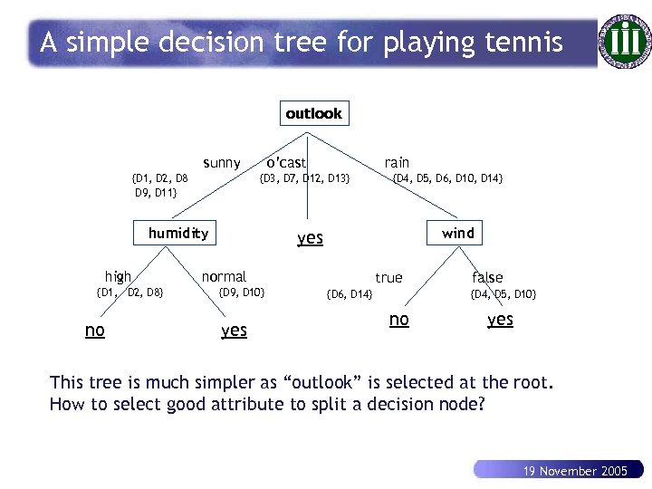A simple decision tree for playing tennis outlook sunny {D 1, D 2, D 8 D 9, D 11} o’cast {D 3, D 7, D 12, D 13} humidity high {D 1, D 2, D 8} no rain {D 4, D 5, D 6, D 10, D 14} wind yes normal {D 9, D 10} yes true {D 6, D 14} false {D 4, D 5, D 10} no yes This tree is much simpler as “outlook” is selected at the root. How to select good attribute to split a decision node? 19 November 2005

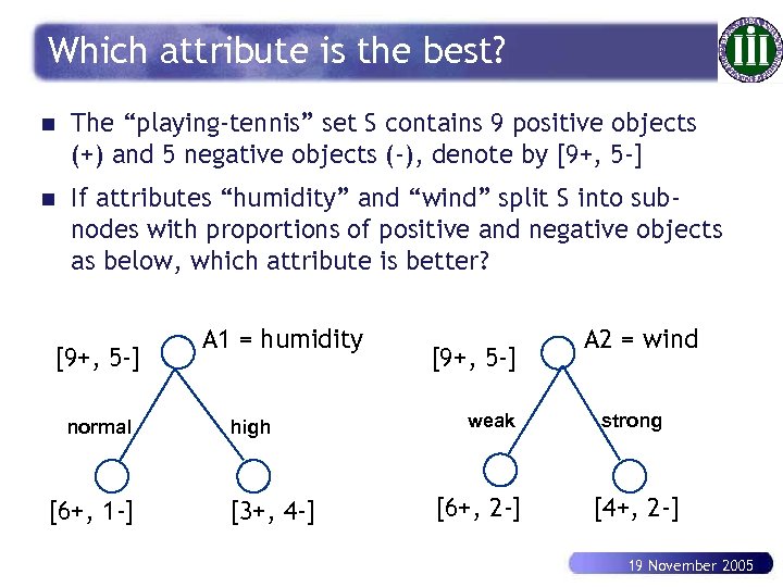Which attribute is the best? n The “playing-tennis” set S contains 9 positive objects (+) and 5 negative objects (-), denote by [9+, 5 -] n If attributes “humidity” and “wind” split S into subnodes with proportions of positive and negative objects as below, which attribute is better? [9+, 5 -] normal [6+, 1 -] A 1 = humidity high [3+, 4 -] [9+, 5 -] weak [6+, 2 -] A 2 = wind strong [4+, 2 -] 19 November 2005

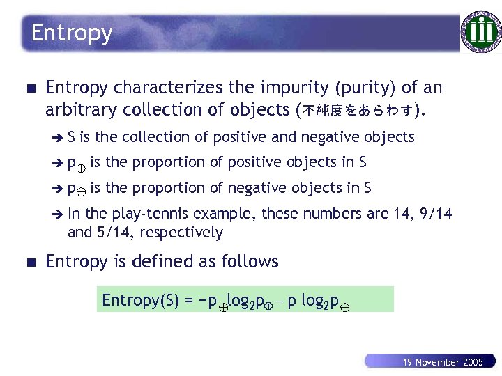Entropy n Entropy characterizes the impurity (purity) of an arbitrary collection of objects (不純度をあらわす). èS is the collection of positive and negative objects èp is the proportion of positive objects in S èp is the proportion of negative objects in S è In the play-tennis example, these numbers are 14, 9/14 and 5/14, respectively n Entropy is defined as follows Entropy(S) = −p log 2 p − p log 2 p 19 November 2005

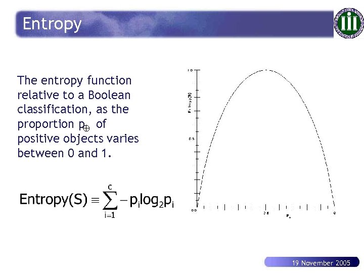Entropy The entropy function relative to a Boolean classification, as the proportion p of positive objects varies between 0 and 1. 19 November 2005

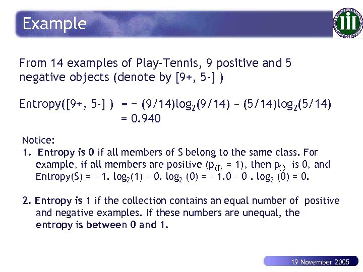Example From 14 examples of Play-Tennis, 9 positive and 5 negative objects (denote by [9+, 5 -] ) Entropy([9+, 5 -] ) = − (9/14)log 2(9/14) = 0. 940 − (5/14)log 2(5/14) Notice: 1. Entropy is 0 if all members of S belong to the same class. For example, if all members are positive (p = 1), then p is 0, and Entropy(S) = − 1. log 2(1) − 0. log 2 (0) = − 1. 0 − 0. log 2 (0) = 0. 2. Entropy is 1 if the collection contains an equal number of positive and negative examples. If these numbers are unequal, the entropy is between 0 and 1. 19 November 2005

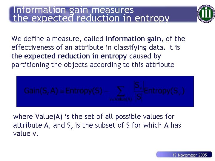Information gain measures the expected reduction in entropy We define a measure, called information gain, of the effectiveness of an attribute in classifying data. It is the expected reduction in entropy caused by partitioning the objects according to this attribute where Value(A) is the set of all possible values for attribute A, and Sv is the subset of S for which A has value v. 19 November 2005

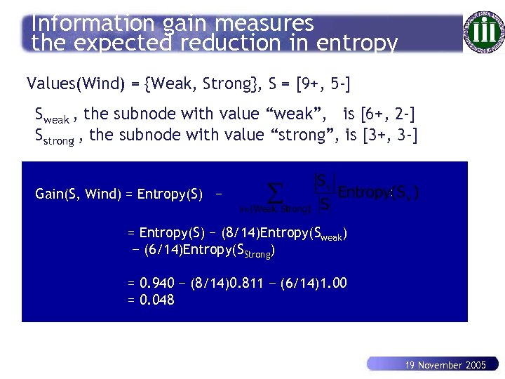Information gain measures the expected reduction in entropy Values(Wind) = {Weak, Strong}, S = [9+, 5 -] Sweak , the subnode with value “weak”, is [6+, 2 -] Sstrong , the subnode with value “strong”, is [3+, 3 -] Gain(S, Wind) = Entropy(S) − (8/14)Entropy(Sweak) − (6/14)Entropy(SStrong) = 0. 940 − (8/14)0. 811 − (6/14)1. 00 = 0. 048 19 November 2005

Which attribute is the best classifier? S: [9+, 5 -] E = 0. 940 Humidity Wind High Normal Weak Strong [3+, 4 -] E = 0. 985 [6+, 1 -] E = 0. 592 [6+, 2 -] E = 0. 811 [3+, 3 -] E = 1. 00 Gain(S, Humidity) =. 940 − (7/14). 985 − (7/14). 592 =. 151 Gain(S, Wind) =. 940 − (8/14). 811 − (6/14)1. 00 =. 048 19 November 2005

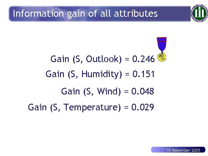Information gain of all attributes Gain (S, Outlook) = 0. 246 Gain (S, Humidity) = 0. 151 Gain (S, Wind) = 0. 048 Gain (S, Temperature) = 0. 029 19 November 2005

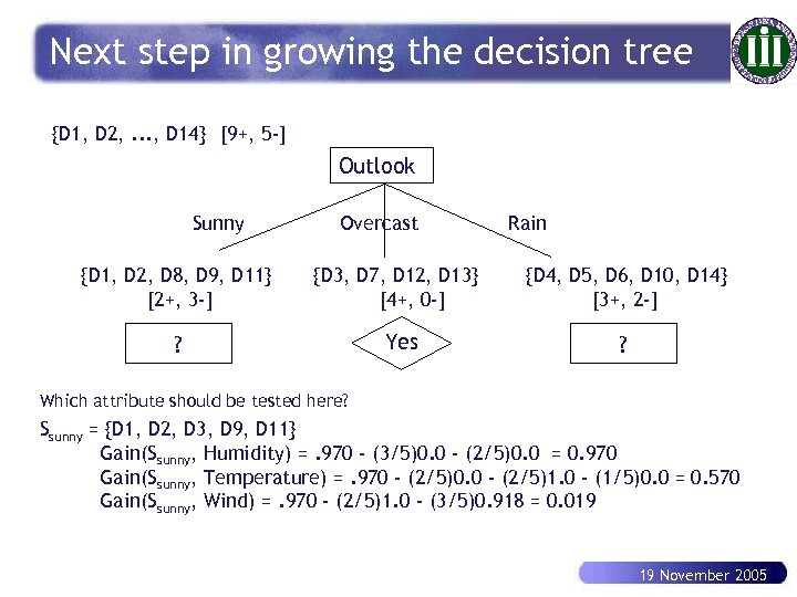Next step in growing the decision tree {D 1, D 2, . . . , D 14} [9+, 5 -] Outlook Sunny Overcast Rain {D 1, D 2, D 8, D 9, D 11} [2+, 3 -] {D 3, D 7, D 12, D 13} [4+, 0 -] {D 4, D 5, D 6, D 10, D 14} [3+, 2 -] ? Yes ? Which attribute should be tested here? Ssunny = {D 1, D 2, D 3, D 9, D 11} Gain(Ssunny, Humidity) =. 970 - (3/5)0. 0 - (2/5)0. 0 = 0. 970 Gain(Ssunny, Temperature) =. 970 - (2/5)0. 0 - (2/5)1. 0 - (1/5)0. 0 = 0. 570 Gain(Ssunny, Wind) =. 970 - (2/5)1. 0 - (3/5)0. 918 = 0. 019 19 November 2005

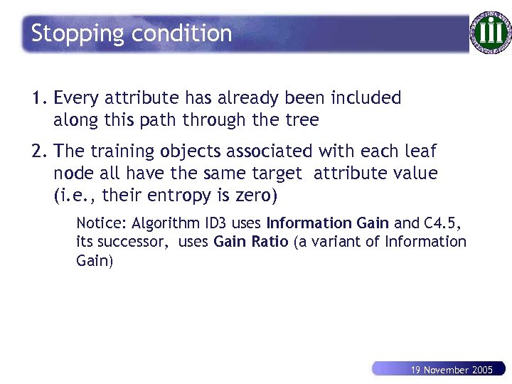Stopping condition 1. Every attribute has already been included along this path through the tree 2. The training objects associated with each leaf node all have the same target attribute value (i. e. , their entropy is zero) Notice: Algorithm ID 3 uses Information Gain and C 4. 5, its successor, uses Gain Ratio (a variant of Information Gain) 19 November 2005

Over-fitting in decision trees n The generated tree may overfit the training data è Too many branches, some may reflect anomalies due to noise or outliers è Result n is in poor accuracy for unseen objects Two approaches to avoid overfitting è Prepruning: Halt tree construction early—do not split a node if this would result in the goodness measure falling below a threshold ð Difficult to choose an appropriate threshold è Postpruning: Remove branches from a “fully grown” tree—get a sequence of progressively pruned trees ð Use a set of data different from the training data to decide which is the “best pruned tree” 19 November 2005

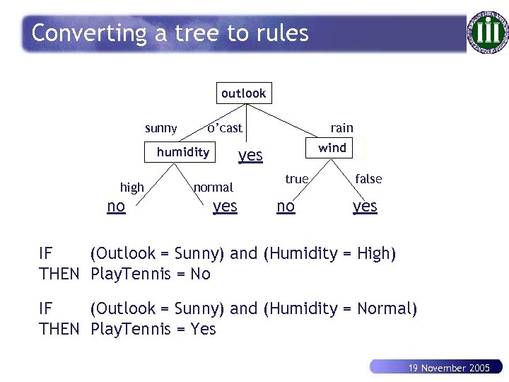Converting a tree to rules outlook sunny o’cast humidity high no rain wind yes normal yes true no false yes IF (Outlook = Sunny) and (Humidity = High) THEN Play. Tennis = No IF (Outlook = Sunny) and (Humidity = Normal) THEN Play. Tennis = Yes 19 November 2005

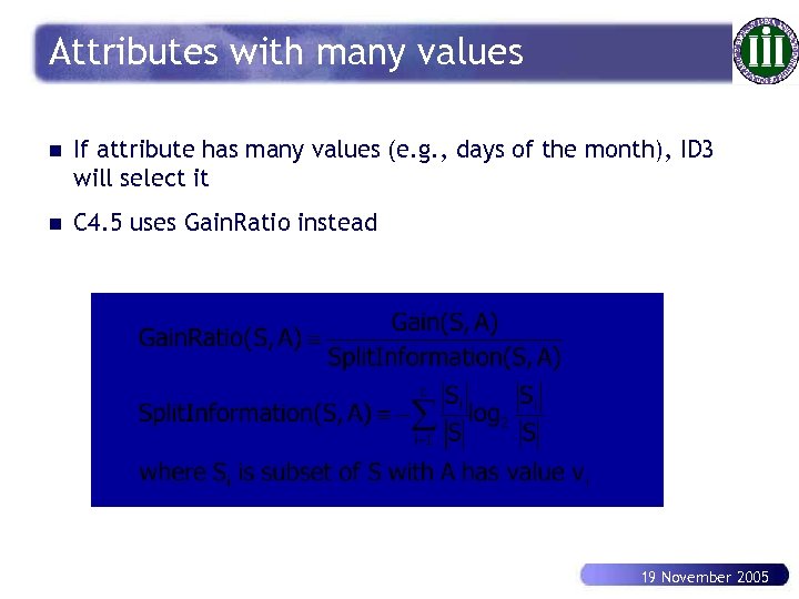Attributes with many values n If attribute has many values (e. g. , days of the month), ID 3 will select it n C 4. 5 uses Gain. Ratio instead 19 November 2005

Bayesian classification Learning statistical classifiers from supervised data basing on Bayes theorem and assumptions on independence/dependence of the data. 19 November 2005

What are Bayesian classification? n Bayesian classifiers are statistical classifiers. Bayesian classification is based on Bayes theorem. n Naïve Bayesian classifiers assume that the effect of an attribute value on a given class is independent of the values of the other attributes. n Bayesian belief networks are graphical models allow the representation of dependencies among subsets of attributes. 19 November 2005

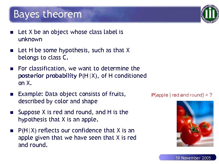Bayes theorem n Let X be an object whose class label is unknown n Let H be some hypothesis, such as that X belongs to class C. n For classification, we want to determine the posterior probability P(H|X), of H conditioned on X. n Example: Data object consists of fruits, described by color and shape n Suppose X is red and round, and H is the hypothesis that X is an apple. n P(H|X) reflects our confidence that X is an apple given that we have seen that X is red and round. P(apple | red and round) = ? 19 November 2005

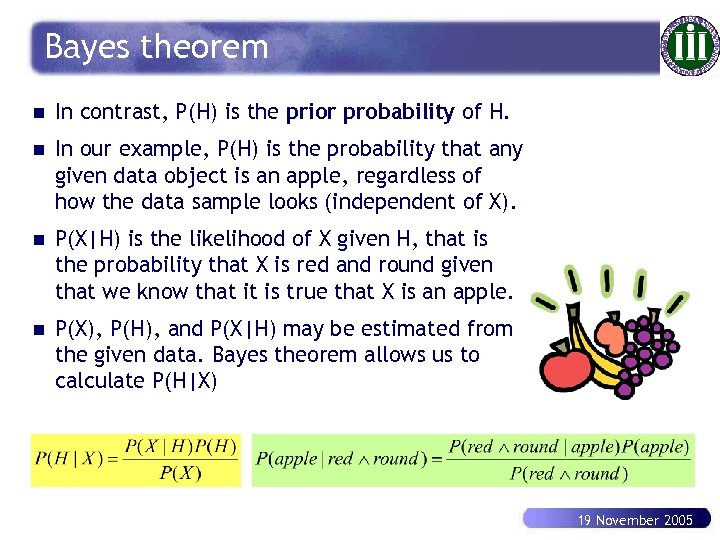Bayes theorem n In contrast, P(H) is the prior probability of H. n In our example, P(H) is the probability that any given data object is an apple, regardless of how the data sample looks (independent of X). n P(X|H) is the likelihood of X given H, that is the probability that X is red and round given that we know that it is true that X is an apple. n P(X), P(H), and P(X|H) may be estimated from the given data. Bayes theorem allows us to calculate P(H|X) 19 November 2005

Naïve Bayesian classification n Suppose X = (x 1, x 2, …, xn), attributes A 1, A 2, …, An n There are m classes C 1, C 2, …, Cm n P(Ci|X) denotes probability that X is classified to class Ci. n Example: P(class = N | outlook=sunny, temperature=hot, humidity=high, wind=strong) n Idea: assign to object X the class label Ci such that P(Ci|X) is maximal, i. e. , P(Ci|X) > P(Cj|X), j, i j. n Ci is called the maximum posterior hypothesis. 19 November 2005

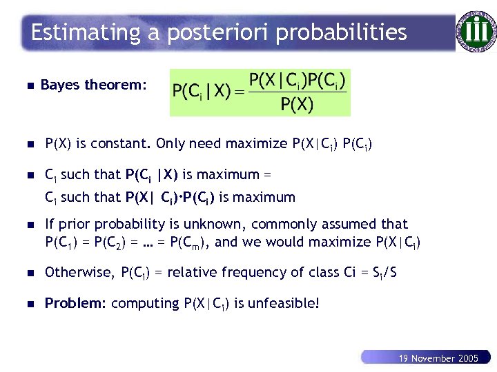Estimating a posteriori probabilities n Bayes theorem: n P(X) is constant. Only need maximize P(X|Ci) P(Ci) n Ci such that P(Ci |X) is maximum = Ci such that P(X| Ci)·P(Ci) is maximum n If prior probability is unknown, commonly assumed that P(C 1) = P(C 2) = … = P(Cm), and we would maximize P(X|Ci) n Otherwise, P(Ci) = relative frequency of class Ci = Si/S n Problem: computing P(X|Ci) is unfeasible! 19 November 2005

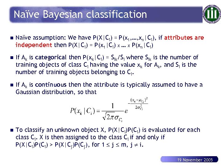Naïve Bayesian classification n Naïve assumption: We have P(X|Ci) = P(x 1, …, xn|Ci), if attributes are independent then P(X|Ci) = P(x 1|Ci) x … x P(xn|Ci) n If Ak is categorical then P(xk|Ci) = Sik/Si where Sik is the number of training objects of class Ci having the value xk for Ak, and Si is the number of training objects belonging to Ci. n If Ak is continuous then the attribute is typically assumed to have a Gaussian distribution, so that n To classify an unknown object X, P(X|Ci)P(Ci) is evaluated for each class Ci. X is then assigned to the class Ci if and only if P(X|Ci)P(Ci) > P(X|Cj)P(Cj), for 1 j m, j i. 19 November 2005

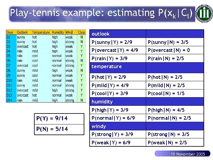Play-tennis example: estimating P(xk|Ci) outlook P(sunny|Y) = 2/9 P(sunny|N) = 3/5 P(overcast|Y) = 4/9 P(overcast|N) = 0 P(rain|Y) = 3/9 P(rain|N) = 2/5 temperature P(hot|Y) = 2/9 P(hot|N) = 2/5 P(mild|Y) = 4/9 P(mild|N) = 2/5 P(cool|Y) = 3/9 P(cool|N) = 1/5 humidity P(high|Y) = 3/9 P(high|N) = 4/5 P(Y) = 9/14 P(normal|Y) = 6/9 P(normal|N) = 2/5 P(N) = 5/14 windy P(strong|Y) = 3/9 P(strong|N) = 3/5 P(weak|Y) = 6/9 P(weak|N) = 2/5 19 November 2005

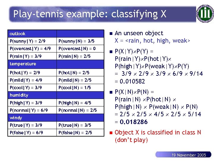Play-tennis example: classifying X n outlook P(sunny|Y) = 2/9 P(overcast|N) = 0 P(rain|Y) = 3/9 P(rain|N) = 2/5 n P(X|Y) P(Y) = P(rain|Y) P(hot|Y) P(high|Y) P(weak|Y) P(Y) = 3/9 2/9 3/9 6/9 9/14 = 0. 010582 n P(X|N) P(N) = P(rain|N) P(hot|N) P(high|N) P(weak|N) P(N) = 2/5 4/5 2/5 5/14 = 0. 018286 n Object X is classified in class N (don’t play) P(sunny|N) = 3/5 P(overcast|Y) = 4/9 An unseen object X = temperature P(hot|Y) = 2/9 P(hot|N) = 2/5 P(mild|Y) = 4/9 P(mild|N) = 2/5 P(cool|Y) = 3/9 P(cool|N) = 1/5 humidity P(high|Y) = 3/9 P(high|N) = 4/5 P(normal|Y) = 6/9 P(normal|N) = 2/5 windy P(true|Y) = 3/9 P(true|N) = 3/5 P(false|Y) = 6/9 P(false|N) = 2/5 19 November 2005

The independence hypothesis n It makes computation possible n It yields optimal classifiers when independence satisfied n But it is seldom satisfied in practice, as attributes (variables) are often correlated n Attempts to overcome this limitation, among others: è Bayesian networks, that combine Bayesian reasoning with causal relationships between attributes è Decision trees, that reason on one attribute at the time, considering most important attributes first 19 November 2005

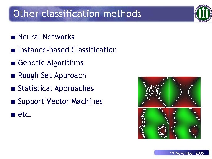Other classification methods n Neural Networks n Instance-based Classification n Genetic Algorithms n Rough Set Approach n Statistical Approaches n Support Vector Machines n etc. 19 November 2005

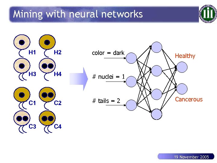Mining with neural networks H 1 H 2 color = dark H 3 H 4 # nuclei = 1 C 2 # tails = 2 C 3 C 4 Healthy Cancerous 19 November 2005

Mining with neural networks n Advantages è è n prediction accuracy is generally high robust, works when training examples contain errors output may be discrete, real-valued, or a vector of several discrete or real-valued attributes fast evaluation of the learned target function Criticism è è è long training time difficult to understand the learned function (weights) not easy to incorporate domain knowledge 19 November 2005

Instance-based classification n Instance-based classification è n Using most similarity individual instances known in the past to classify a new instance Typical approaches è k-nearest neighbor approach ð è Locally weighted regression ð è Instances as points in an Euclidean space Constructs local approximation Case-based reasoning ð Uses symbolic representations and knowledge-based inference 19 November 2005

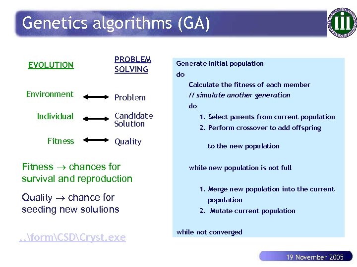Genetics algorithms (GA) EVOLUTION PROBLEM SOLVING Generate initial population do Calculate the fitness of each member Environment Individual Fitness Problem Candidate Solution Quality Fitness chances for survival and reproduction Quality chance for seeding new solutions . . formCSDCryst. exe // simulate another generation do 1. Select parents from current population 2. Perform crossover to add offspring to the new population while new population is not full 1. Merge new population into the current population 2. Mutate current population while not converged 19 November 2005

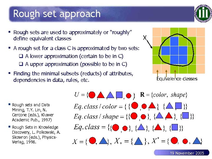Rough set approach § Rough sets are used to approximately or “roughly” X define equivalent classes § A rough set for a class C is approximated by two sets: q A lower approximation (certain to be in C) q A upper approximation (possible to be in C) § Finding the minimal subsets (reducts) of attributes, Equivalence classes dependencies in data, rules, etc. , , , § Rough sets and Data § Rough Sets in Knowledge Discovery, L. Polkowski, A. Skowron (eds. ), Physica. Verlag, 1998. , , Mining, T. Y. Lin, N. Cercone (eds. ), Kluwer Academic Pub. , 1997) , , , 19 November 2005

Association rule mining Description learning that aims to find all possible associations from data. 19 November 2005

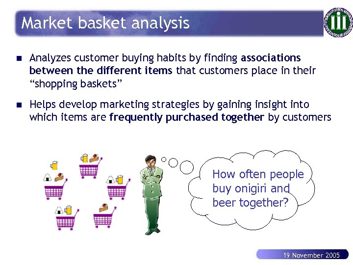Market basket analysis n Analyzes customer buying habits by finding associations between the different items that customers place in their “shopping baskets” n Helps develop marketing strategies by gaining insight into which items are frequently purchased together by customers How often people buy onigiri and beer together? 19 November 2005

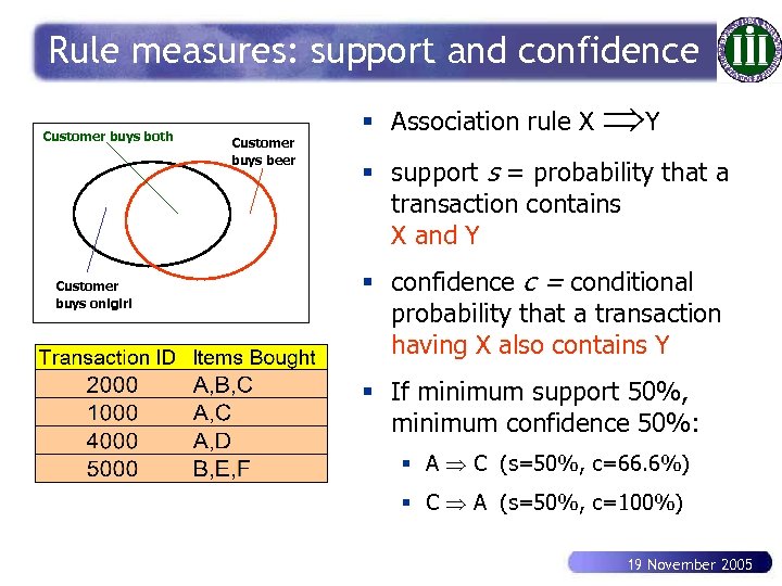Rule measures: support and confidence Customer buys both Customer buys onigiri Customer buys beer § Association rule X Y § support s = probability that a transaction contains X and Y § confidence c = conditional probability that a transaction having X also contains Y § If minimum support 50%, minimum confidence 50%: § A C (s=50%, c=66. 6%) § C A (s=50%, c=100%) 19 November 2005

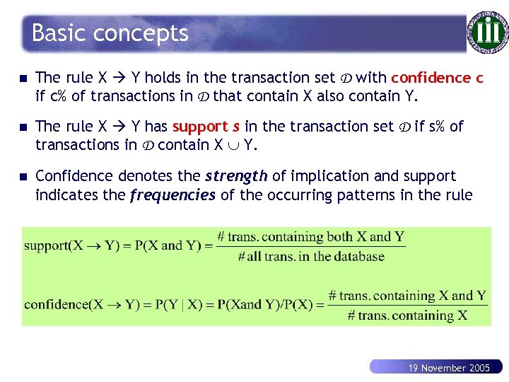Basic concepts n The rule X Y holds in the transaction set D with confidence c if c% of transactions in D that contain X also contain Y. n The rule X Y has support s in the transaction set D if s% of transactions in D contain X Y. n Confidence denotes the strength of implication and support indicates the frequencies of the occurring patterns in the rule 19 November 2005

Association mining: Apriori algorithm It is composed of two steps: 1. Find all frequent itemsets: By definition, each of these itemsets will occur at least as frequently as a pre-determined minimum support count 2. Generate strong association rules from the frequent itemsets: By definition, these rules must satisfy minimum support and minimum confidence 19 November 2005

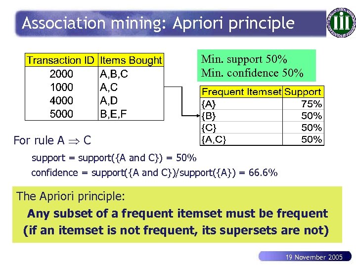Association mining: Apriori principle Min. support 50% Min. confidence 50% For rule A C support = support({A and C}) = 50% confidence = support({A and C})/support({A}) = 66. 6% The Apriori principle: Any subset of a frequent itemset must be frequent (if an itemset is not frequent, its supersets are not) 19 November 2005

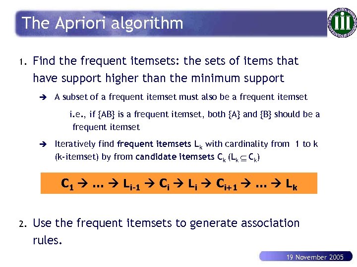The Apriori algorithm 1. Find the frequent itemsets: the sets of items that have support higher than the minimum support è A subset of a frequent itemset must also be a frequent itemset i. e. , if {AB} is a frequent itemset, both {A} and {B} should be a frequent itemset è Iteratively find frequent itemsets Lk with cardinality from 1 to k (k-itemset) by from candidate itemsets Ck (Lk Ck) C 1 … Li-1 Ci Li Ci+1 … Lk 2. Use the frequent itemsets to generate association rules. 19 November 2005

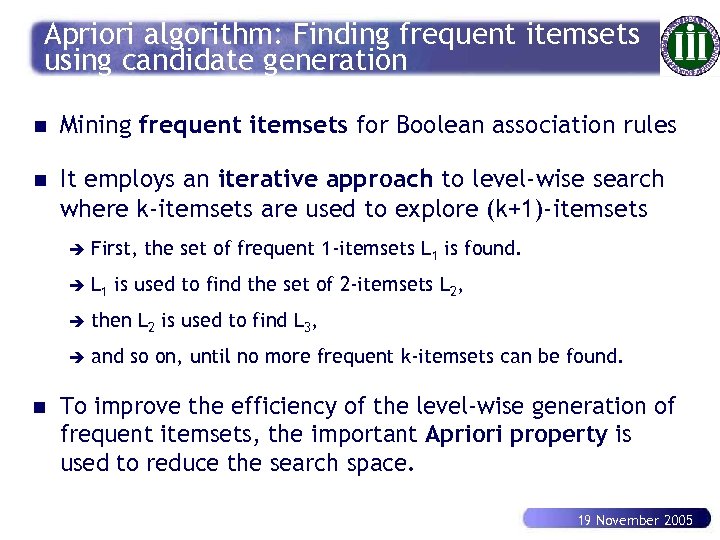Apriori algorithm: Finding frequent itemsets using candidate generation n Mining frequent itemsets for Boolean association rules n It employs an iterative approach to level-wise search where k-itemsets are used to explore (k+1)-itemsets è è L 1 is used to find the set of 2 -itemsets L 2, è then L 2 is used to find L 3, è n First, the set of frequent 1 -itemsets L 1 is found. and so on, until no more frequent k-itemsets can be found. To improve the efficiency of the level-wise generation of frequent itemsets, the important Apriori property is used to reduce the search space. 19 November 2005

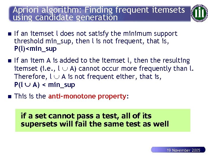Apriori algorithm: Finding frequent itemsets using candidate generation n If an itemset l does not satisfy the minimum support threshold min_sup, then l is not frequent, that is, P(l)

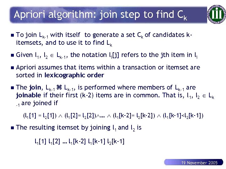Apriori algorithm: join step to find Ck n To join Lk-1 with itself to generate a set Ck of candidates kitemsets, and to use it to find Lk n Given l 1, l 2 Lk-1, the notation li[j] refers to the jth item in li n Apriori assumes that items within a transaction or itemset are sorted in lexicographic order n The join, Lk-1, is performed where members of Lk-1 are joinable if their first (k-2) items are in common. That is, l 1, l 2 Lk -1 are joined if (l 1[1] = l 2[1]) (l 1[2]= l 2[2]) … (l 1[k-2]= l 2[k-2]) (l 1[k-1]

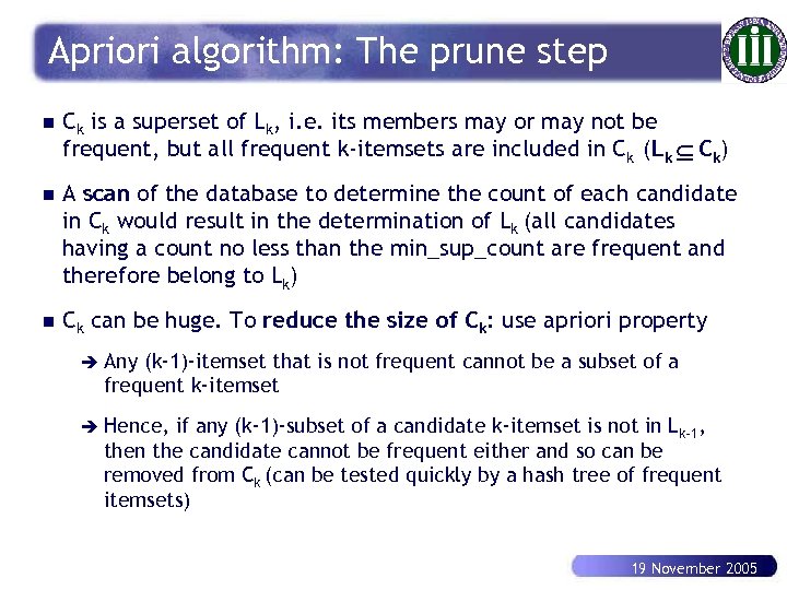Apriori algorithm: The prune step n Ck is a superset of Lk, i. e. its members may or may not be frequent, but all frequent k-itemsets are included in Ck (Lk Ck) n A scan of the database to determine the count of each candidate in Ck would result in the determination of Lk (all candidates having a count no less than the min_sup_count are frequent and therefore belong to Lk) n Ck can be huge. To reduce the size of Ck: use apriori property è Any (k-1)-itemset that is not frequent cannot be a subset of a frequent k-itemset è Hence, if any (k-1)-subset of a candidate k-itemset is not in Lk-1, then the candidate cannot be frequent either and so can be removed from Ck (can be tested quickly by a hash tree of frequent itemsets) 19 November 2005

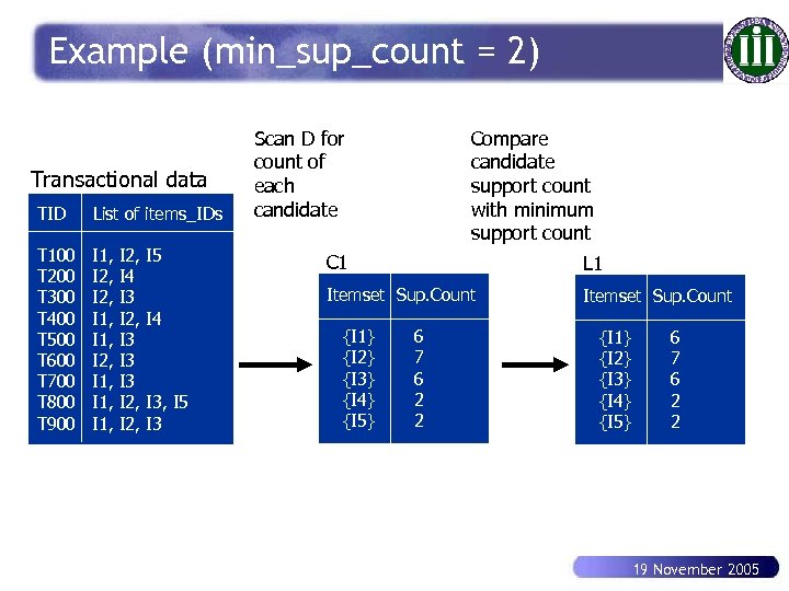Example (min_sup_count = 2) Transactional data TID List of items_IDs T 100 T 200 T 300 T 400 T 500 T 600 T 700 T 800 T 900 I 1, I 2, I 1, I 2, I 4 I 3 I 2, I 3 I 3 I 2, I 5 Scan D for count of each candidate Compare candidate support count with minimum support count I 3, I 5 I 3 L 1 Itemset Sup. Count I 4 C 1 Itemset Sup. Count {I 1} {I 2} {I 3} {I 4} {I 5} 6 7 6 2 2 19 November 2005

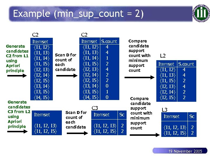Example (min_sup_count = 2) C 2 Itemset Generate {I 1, I 2} candidates {I 1, I 3} C 2 from L 1 {I 1, I 4} using {I 1, I 5} Apriori {I 2, I 3} principle {I 2, I 4} {I 2, I 5} {I 3, I 4} {I 3, I 5} {I 4, I 5} C 2 Scan D for count of each candidate Generate candidates C 3 from L 2 Itemset using Apriori {I 1, I 2, I 3} principle {I 1, I 2, I 5} Itemset S. count {I 1, I 2} 4 {I 1, I 3} 4 {I 1, I 4} 1 {I 1, I 5} 2 {I 2, I 3} 4 {I 2, I 4} 2 {I 2, I 5} 2 {I 3, I 4} 0 {I 3, I 5} 1 {I 4, I 5} 0 Scan D for count of each candidate Compare candidate support count with minimum support count C 3 Itemset Sc {I 1, I 2, I 3} 2 {I 1, I 2, I 5} 2 Compare candidate support count with minimum support count L 2 Itemset S. count {I 1, I 2} 4 {I 1, I 3} 4 {I 1, I 5} 2 {I 2, I 3} 4 {I 2, I 4} 2 {I 2, I 5} 2 L 3 Itemset Sc {I 1, I 2, I 3} 2 {I 1, I 2, I 5} 2 19 November 2005

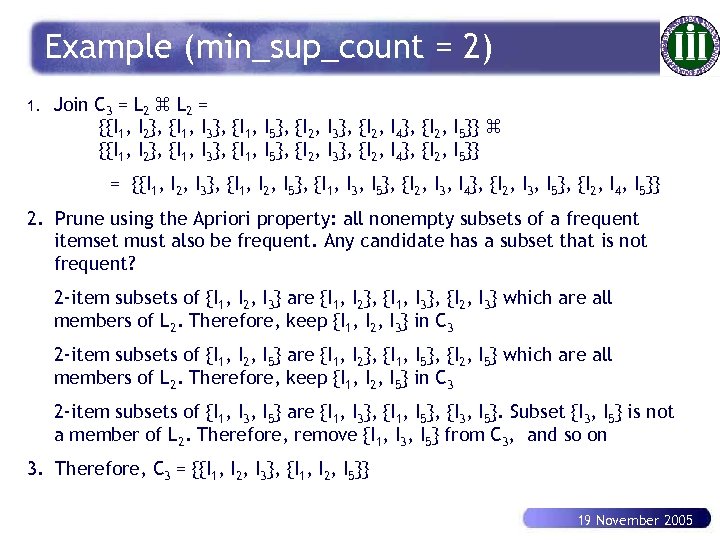Example (min_sup_count = 2) 1. Join C 3 = L 2 = {{I 1, I 2}, {I 1, I 3}, {I 1, I 5}, {I 2, I 3}, {I 2, I 4}, {I 2, I 5}} = {{I 1, I 2, I 3}, {I 1, I 2, I 5}, {I 1, I 3, I 5}, {I 2, I 3, I 4}, {I 2, I 3, I 5}, {I 2, I 4, I 5}} 2. Prune using the Apriori property: all nonempty subsets of a frequent itemset must also be frequent. Any candidate has a subset that is not frequent? 2 -item subsets of {I 1, I 2, I 3} are {I 1, I 2}, {I 1, I 3}, {I 2, I 3} which are all members of L 2. Therefore, keep {I 1, I 2, I 3} in C 3 2 -item subsets of {I 1, I 2, I 5} are {I 1, I 2}, {I 1, I 5}, {I 2, I 5} which are all members of L 2. Therefore, keep {I 1, I 2, I 5} in C 3 2 -item subsets of {I 1, I 3, I 5} are {I 1, I 3}, {I 1, I 5}, {I 3, I 5}. Subset {I 3, I 5} is not a member of L 2. Therefore, remove {I 1, I 3, I 5} from C 3, and so on 3. Therefore, C 3 = {{I 1, I 2, I 3}, {I 1, I 2, I 5}} 19 November 2005

Cluster analysis Description learning that aims to detect and groups of similar objects from unsupervised data. 19 November 2005

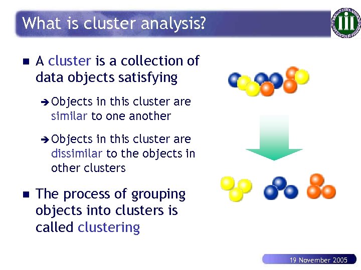What is cluster analysis? n A cluster is a collection of data objects satisfying è Objects in this cluster are similar to one another è Objects in this cluster are dissimilar to the objects in other clusters n The process of grouping objects into clusters is called clustering 19 November 2005

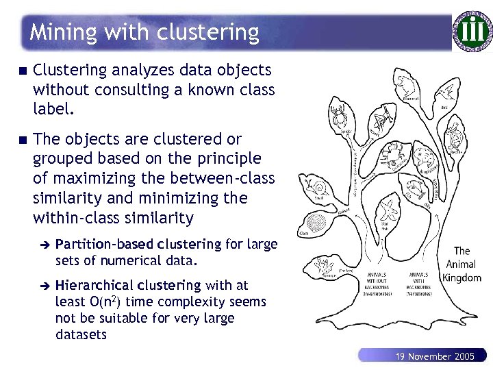Mining with clustering n Clustering analyzes data objects without consulting a known class label. n The objects are clustered or grouped based on the principle of maximizing the between-class similarity and minimizing the within-class similarity è Partition-based clustering for large sets of numerical data. è Hierarchical clustering with at least O(n 2) time complexity seems not be suitable for very large datasets 19 November 2005

What is good clustering? n A good clustering method will produce high quality clusters with è high intra-class similarity (within a class) è low inter-class similarity (between classes) n The quality of clustering basically depends on the similarity measure and the cluster representative used by the method n New forms of clustering require different criteria of quality. 19 November 2005

Clustering in different fields n Statistics: since many years, focus on distancebased clustering (S-Plus, SPSS, SAS) n Machine learning: unsupervised learning. In conceptual clustering, a group of objects forms a class only if it is described by a concept n KDD: Efficient and effective clustering of large databases: scalability, complex shapes and types of data, high dimensional clustering, mixed numerical and categorical data 19 November 2005

Typical requirements of clustering n Scalability n Ability to deal with different types of attributes n Discovery of clusters with arbitrary shape n Minimal requirements for domain knowledge to determine input parameters n Ability to deal with noisy data n Insensitivity to the order of input records n High dimensionality n Constraint-based clustering n Interpretability and usability 19 November 2005

Clustering methods in KDD n Partitioning Methods n Hierarchical Methods n Density-Based Methods n Grid-Based Methods n Model-Based Methods 19 November 2005

Partitioning methods n Given n objects and k as number of clusters to form. A partitioning algorithm organizes the objects into a partition of k clusters n The clusters are formed to optimize an objective partitioning criterion so that the objects within a cluster are “similar” , whereas the objects of different classes are “dissimilar” n C: STATSTA_WIN. EXE 19 November 2005

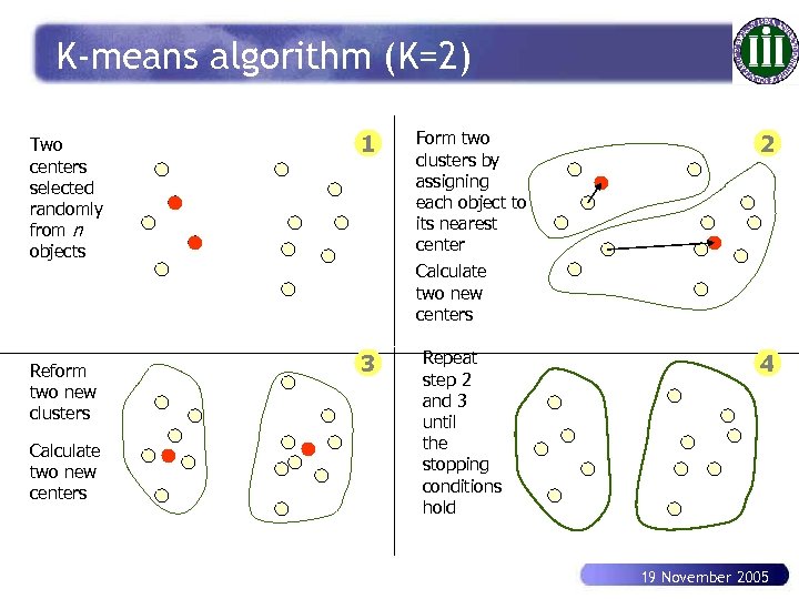K-means algorithm (K=2) Two centers selected randomly from n objects Reform two new clusters Calculate two new centers 1 3 Form two clusters by assigning each object to its nearest center Calculate two new centers Repeat step 2 and 3 until the stopping conditions hold 2 4 19 November 2005

Partitioning methods n The k-means algorithm is sensitive to outliers n The k-medoids method uses medoid (the most centrally located object in a cluster) n The EM (Expectation Maximization) algorithm: assigns to a cluster according to a weight representing the probability of membership. n PAM (Partitioning Around Medoids) n From k-Medoids to CLARA (Clustering LARge Applications) n From CLARA to CLARANS (Clustering LARge Applications based on RANdomized Search) 19 November 2005

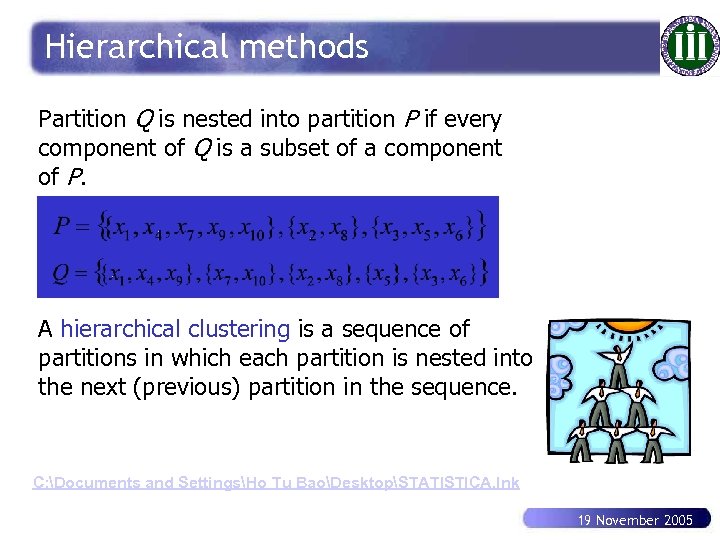Hierarchical methods Partition Q is nested into partition P if every component of Q is a subset of a component of P. A hierarchical clustering is a sequence of partitions in which each partition is nested into the next (previous) partition in the sequence. C: Documents and SettingsHo Tu BaoDesktopSTATISTICA. lnk 19 November 2005

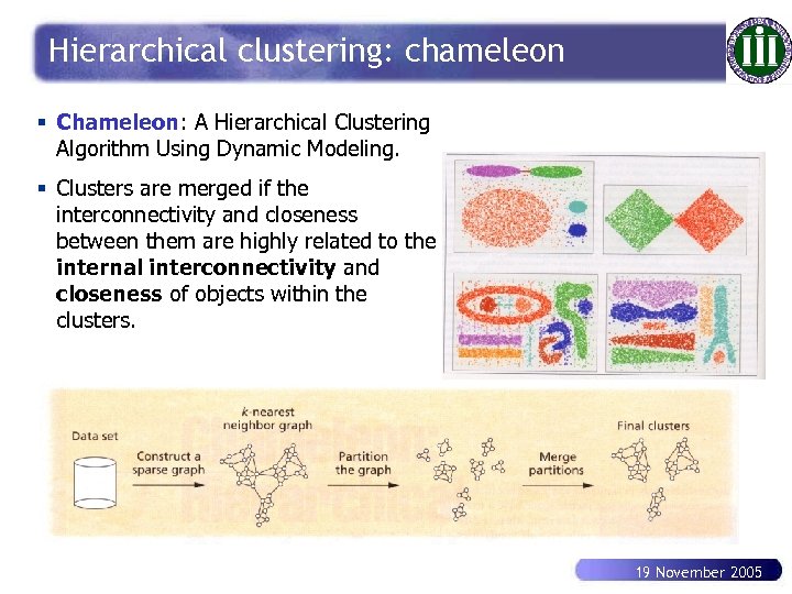Hierarchical clustering: chameleon § Chameleon: A Hierarchical Clustering Algorithm Using Dynamic Modeling. § Clusters are merged if the interconnectivity and closeness between them are highly related to the internal interconnectivity and closeness of objects within the clusters. 19 November 2005

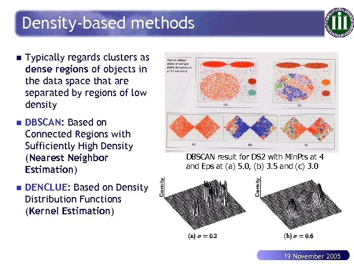Density-based methods n Typically regards clusters as dense regions of objects in the data space that are separated by regions of low density n DBSCAN: Based on Connected Regions with Sufficiently High Density (Nearest Neighbor Estimation) n DBSCAN result for DS 2 with Min. Pts at 4 and Eps at (a) 5. 0, (b) 3. 5 and (c) 3. 0 DENCLUE: Based on Density Distribution Functions (Kernel Estimation) 19 November 2005

Text mining Finding unknown useful information from huge collection of textual data. 19 November 2005

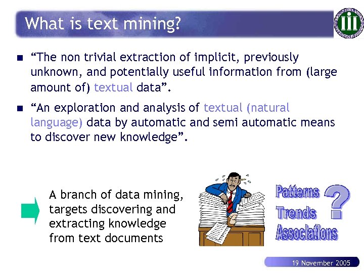What is text mining? n “The non trivial extraction of implicit, previously unknown, and potentially useful information from (large amount of) textual data”. n “An exploration and analysis of textual (natural language) data by automatic and semi automatic means to discover new knowledge”. A branch of data mining, targets discovering and extracting knowledge from text documents 19 November 2005

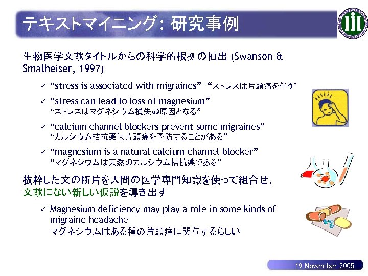テキストマイニング: 研究事例 生物医学文献タイトルからの科学的根拠の抽出 (Swanson & Smalheiser, 1997) ü “stress is associated with migraines”　“ストレスは片頭痛を伴う” ü “stress can lead to loss of magnesium”　　　　　 “ストレスはマグネシウム損失の原因となる” ü “calcium channel blockers prevent some migraines”　　　　　　　 “カルシウム拮抗薬は片頭痛を予防することがある” ü “magnesium is a natural calcium channel blocker”　　　　　　　 “マグネシウムは天然のカルシウム拮抗薬である” 抜粋した文の断片を人間の医学専門知識を使って組合せ， 文献にない新しい仮説を導き出す ü Magnesium deficiency may play a role in some kinds of migraine headache　　　　　　　 マグネシウムはある種の片頭痛に関与するらしい 19 November 2005

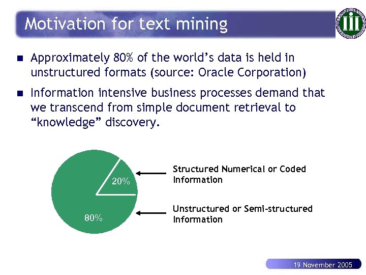Motivation for text mining n Approximately 80% of the world’s data is held in unstructured formats (source: Oracle Corporation) n Information intensive business processes demand that we transcend from simple document retrieval to “knowledge” discovery. 20% 80% Structured Numerical or Coded Information Unstructured or Semi-structured Information 19 November 2005

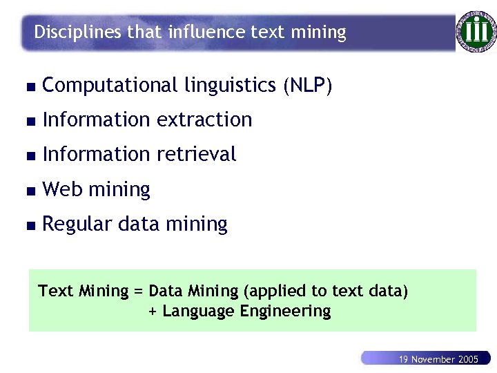Disciplines that influence text mining n Computational linguistics (NLP) n Information extraction n Information retrieval n Web mining n Regular data mining Text Mining = Data Mining (applied to text data) + Language Engineering 19 November 2005

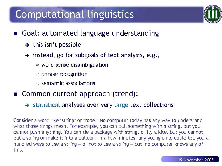Computational linguistics n Goal: automated language understanding è this isn’t possible è instead, go for subgoals of text analysis, e. g. , ð ð phrase recognition ð n word sense disambiguation semantic associations Common current approach (trend): è statistical analyses over very large text collections Consider a word like "string" or "rope. " No computer today has any way to understand what those things mean. For example, you can pull something with a string, but you cannot push anything. You can tie a package with string, or fly a kite, but you cannot eat a string or make it into a balloon. In a few minutes, any young child could tell you a hundred ways to use a string or not to use a string but no computer knows any of this. 19 November 2005

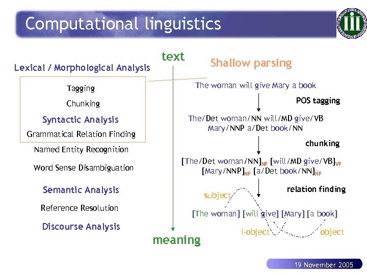Computational linguistics Lexical / Morphological Analysis Tagging text Shallow parsing The woman will give Mary a book POS tagging Chunking Syntactic Analysis Grammatical Relation Finding The/Det woman/NN will/MD give/VB Mary/NNP a/Det book/NN chunking Named Entity Recognition Word Sense Disambiguation [The/Det woman/NN]NP [will/MD give/VB]VP [Mary/NNP]NP [a/Det book/NN]NP Semantic Analysis Reference Resolution relation finding subject [The woman] [will give] [Mary] [a book] Discourse Analysis meaning i-object 19 November 2005

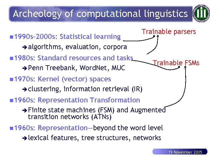Archeology of computational linguistics n 1990 s– 2000 s: Statistical learning è algorithms, evaluation, corpora Trainable parsers n 1980 s: Standard resources and tasks è Penn Treebank, Word. Net, MUC Trainable FSMs n 1970 s: Kernel (vector) spaces è clustering, information retrieval (IR) n 1960 s: Representation Transformation è Finite state machines (FSM) and Augmented transition networks (ATNs) n 1960 s: Representation—beyond the word level è lexical features, tree structures, networks 19 November 2005

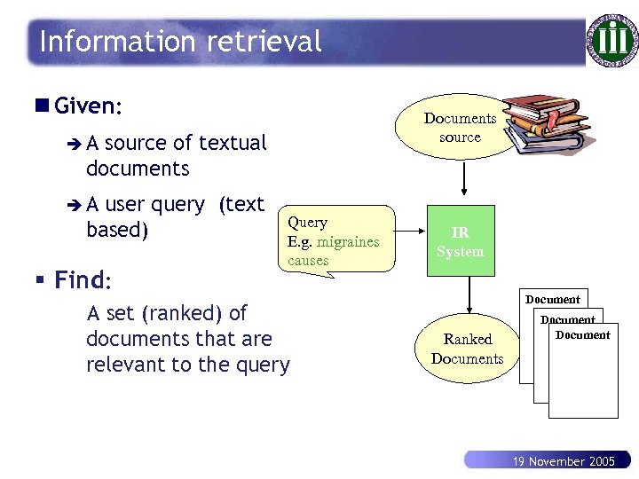Information retrieval n Given: Documents source èA source of textual documents èA user query (text based) § Find: Query E. g. migraines causes A set (ranked) of documents that are relevant to the query IR System Document Ranked Documents Document 19 November 2005

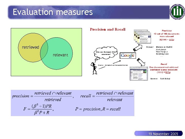Evaluation measures retrieved relevant 19 November 2005

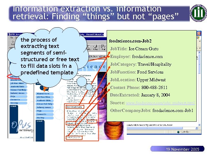Information extraction vs. information retrieval: Finding “things” but not “pages” the process of extracting text segments of semistructured or free text to fill data slots in a predefined template foodscience. com-Job 2 Job. Title: Ice Cream Guru Employer: foodscience. com Job. Category: Travel/Hospitality Job. Function: Food Services Job. Location: Upper Midwest Contact Phone: 800 -488 -2611 Date. Extracted: January 8, 2004 Source: www. foodscience. com/jobs_midwest. html Other. Company. Jobs: foodscience. com-Job 1 19 November 2005

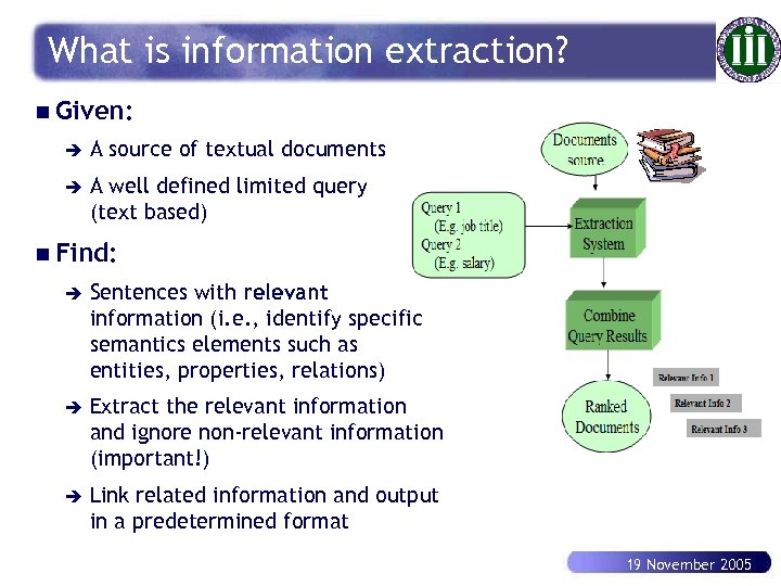What is information extraction? n Given: è A source of textual documents è A well defined limited query (text based) n Find: è Sentences with relevant information (i. e. , identify specific semantics elements such as entities, properties, relations) è Extract the relevant information and ignore non-relevant information (important!) è Link related information and output in a predetermined format 19 November 2005

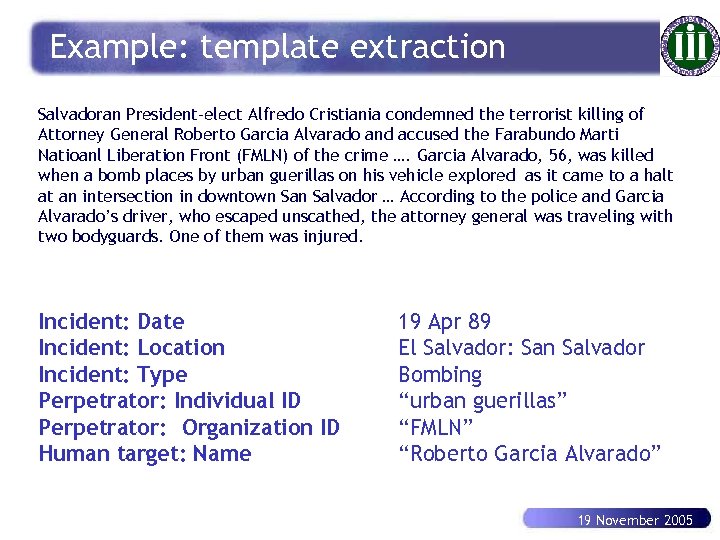Example: template extraction Salvadoran President-elect Alfredo Cristiania condemned the terrorist killing of Attorney General Roberto Garcia Alvarado and accused the Farabundo Marti Natioanl Liberation Front (FMLN) of the crime …. Garcia Alvarado, 56, was killed when a bomb places by urban guerillas on his vehicle explored as it came to a halt at an intersection in downtown Salvador … According to the police and Garcia Alvarado’s driver, who escaped unscathed, the attorney general was traveling with two bodyguards. One of them was injured. Incident: Date Incident: Location Incident: Type Perpetrator: Individual ID Perpetrator: Organization ID Human target: Name 19 Apr 89 El Salvador: San Salvador Bombing “urban guerillas” “FMLN” “Roberto Garcia Alvarado” 19 November 2005

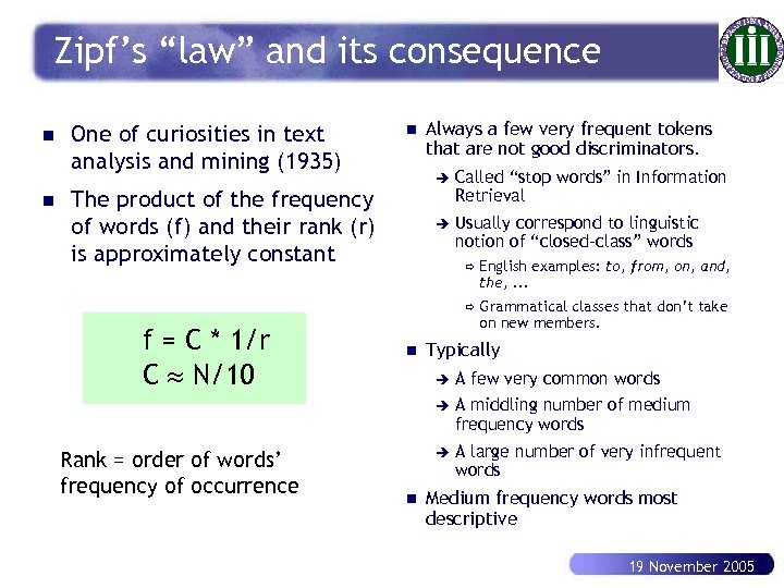Zipf’s “law” and its consequence n n One of curiosities in text analysis and mining (1935) n Always a few very frequent tokens that are not good discriminators. è è The product of the frequency of words (f) and their rank (r) is approximately constant Called “stop words” in Information Retrieval Usually correspond to linguistic notion of “closed-class” words n English examples: to, from, on, and, the, . . . ð f = C * 1/r C N/10 ð Grammatical classes that don’t take on new members. Typically A middling number of medium frequency words è n A few very common words è Rank = order of words’ frequency of occurrence è A large number of very infrequent words Medium frequency words most descriptive 19 November 2005

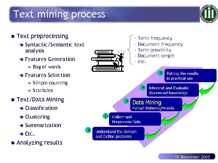Text mining process n Text preprocessing è Syntactic/Semantic analysis è Features ð Generation Bag of words è Features Selection ð Simple counting ð n text - Term frequency - Document frequency - Term proximity - Document length - etc. Statistics Text/Data Mining è Classification è Clustering è Summarization è Etc. n Analyzing results 19 November 2005

Typical issues and techniques n Text Categorization (text classification) n Text Clustering n Text Summarization n Trend Detection n Relationship Analysis n Information Extraction n Question-Answering n Text Visualization n etc. 19 November 2005

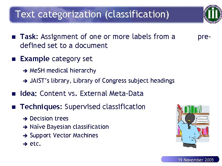Text categorization (classification) n Task: Assignment of one or more labels from a defined set to a document n Example category set è Me. SH medical hierarchy è pre- JAIST’s library, Library of Congress subject headings n Idea: Content vs. External Meta-Data n Techniques: Supervised classification Decision trees è Naïve Bayesian classification è Support Vector Machines è etc. è 19 November 2005

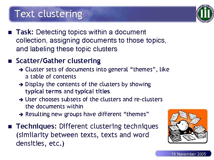Text clustering n Task: Detecting topics within a document collection, assigning documents to those topics, and labeling these topic clusters n Scatter/Gather clustering Cluster sets of documents into general “themes”, like a table of contents è Display the contents of the clusters by showing typical terms and typical titles è User chooses subsets of the clusters and re-clusters the documents within è Resulting new groups have different “themes” è n Techniques: Different clustering techniques (similarity between texts, texts and word densities, etc. ) 19 November 2005

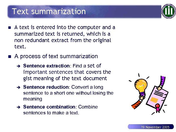Text summarization n A text is entered into the computer and a summarized text is returned, which is a non redundant extract from the original text. n A process of text summarization è Sentence extraction: Find a set of important sentences that covers the gist meaning of the text document è Sentence reduction: Convert a long sentence to a short one without losing the meaning è Sentence combination: Combine sentences to make a text. 19 November 2005

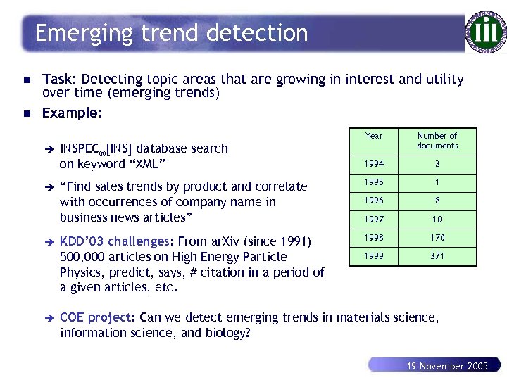Emerging trend detection n n Task: Detecting topic areas that are growing in interest and utility over time (emerging trends) Example: Year è è Number of documents 1994 3 “Find sales trends by product and correlate with occurrences of company name in business news articles” 1995 1 1996 8 1997 10 KDD’ 03 challenges: From ar. Xiv (since 1991) 500, 000 articles on High Energy Particle Physics, predict, says, # citation in a period of a given articles, etc. 1998 170 1999 371 INSPEC®[INS] database search on keyword “XML” COE project: Can we detect emerging trends in materials science, information science, and biology? 19 November 2005

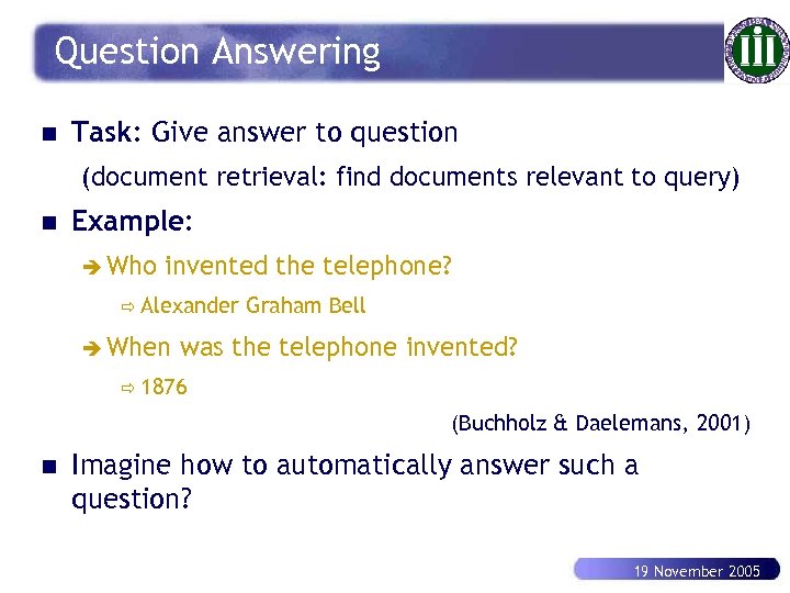Question Answering n Task: Give answer to question (document retrieval: find documents relevant to query) n Example: è Who invented the telephone? ð Alexander è When Graham Bell was the telephone invented? ð 1876 (Buchholz & Daelemans, 2001) n Imagine how to automatically answer such a question? 19 November 2005

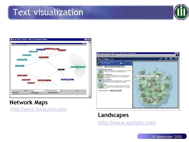Text visualization Network Maps http: //www. lexiquest. com Landscapes http: //www. aurigin. com 19 November 2005

Web mining Finding unknown useful information from the World Wide Web. 19 November 2005

Data Mining and Web Mining n Data mining turns data into knowledge. n Web mining is to apply data mining techniques to extract and uncover knowledge from web documents and services. 19 November 2005

WWW specifics n Web: èA huge, widely-distributed è Highly heterogeneous è Semi-structured è Hypertext/hypermedia è Interconnected n information repository Web is a huge collection of documents plus è Hyper-link è Access information and usage information 19 November 2005

Web user tasks n Finding relevant information è è n The user usually uses a simple keyword query and receive a list of ranked pages Current problem: low precision (irrelevance of search result), and low recall (inability to index all the information on the Web) Creating new knowledge over the existing data è n Personalizing the information è n Want to extract knowledge from Web data (assuming to have it) People differ in the contents and presentations they prefer while interacting with the Web Learning about consumers and individual users è Knowing what the customers do and want 19 November 2005

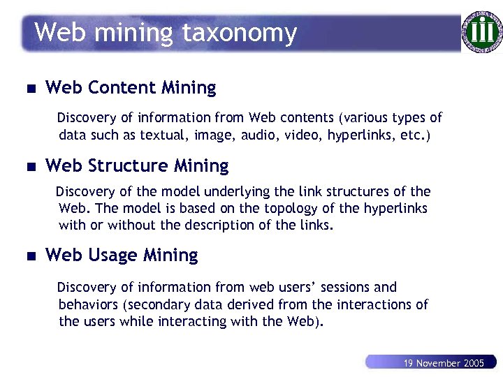Web mining taxonomy n Web Content Mining Discovery of information from Web contents (various types of data such as textual, image, audio, video, hyperlinks, etc. ) n Web Structure Mining Discovery of the model underlying the link structures of the Web. The model is based on the topology of the hyperlinks with or without the description of the links. n Web Usage Mining Discovery of information from web users’ sessions and behaviors (secondary data derived from the interactions of the users while interacting with the Web). 19 November 2005

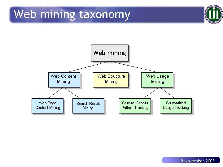Web mining taxonomy Web Mining Web mining Web Content Mining Web Page Content Mining Web Structure Mining Search Result Mining Web Usage Mining General Access Pattern Tracking Customized Usage Tracking 19 November 2005

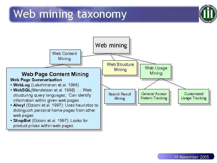Web mining taxonomy Web mining Web. Mining Web Content Mining Web Page Summarization • Web. Log (Lakshmanan et. al. 1996) • Web. SQL(Mendelzon et. al. 1998) …: Web structuring query languages; Can identify information within given web pages • Ahoy! (Etzioni et. al. 1997): Uses heuristics to distinguish personal home pages from other web pages • Shop. Bot (Etzioni et. al. 1997): Looks for product prices within web pages Web Structure Mining Search Result Mining Web Usage Mining General Access Pattern Tracking Customized Usage Tracking 19 November 2005

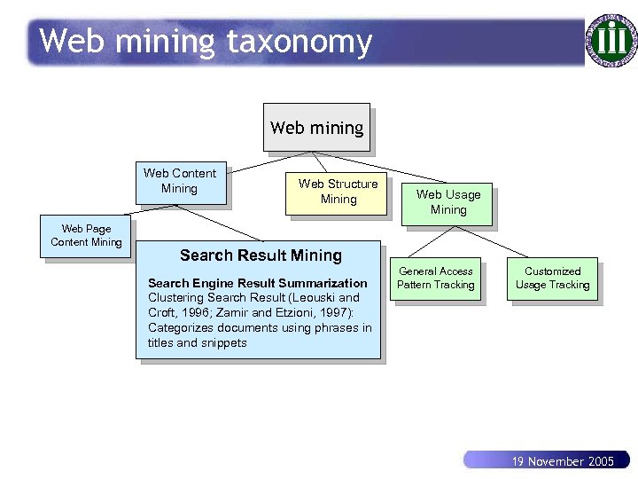Web mining taxonomy Web mining Web. Mining Web Content Mining Web Page Content Mining Web Structure Mining Web Usage Mining Search Result Mining Search Engine Result Summarization Clustering Search Result (Leouski and Croft, 1996; Zamir and Etzioni, 1997): Categorizes documents using phrases in titles and snippets General Access Pattern Tracking Customized Usage Tracking 19 November 2005

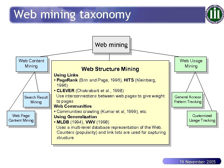Web mining taxonomy Web mining Web. Mining Web Content Mining Search Result Mining Web Page Content Mining Web Structure Mining Using Links • Page. Rank (Brin and Page, 1996), HITS (Kleinberg, 1996) • CLEVER (Chakrabarti et al. , 1998) Use interconnections between web pages to give weight to pages Web Communities • Communities crawling (Kumar et al, 1999), etc. Using Generalization • MLDB (1994), VWV (1998) Uses a multi-level database representation of the Web. Counters (popularity) and link lists are used for capturing structure. Web Usage Mining General Access Pattern Tracking Customized Usage Tracking 19 November 2005

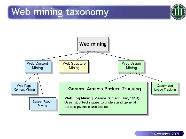Web mining taxonomy Web mining Web. Mining Web Content Mining Web Page Content Mining Search Result Mining Web Structure Mining Web Usage Mining General Access Pattern Tracking Customized Usage Tracking • Web Log Mining (Zaïane, Xin and Han, 1998) Uses KDD techniques to understand general access patterns and trends. 19 November 2005

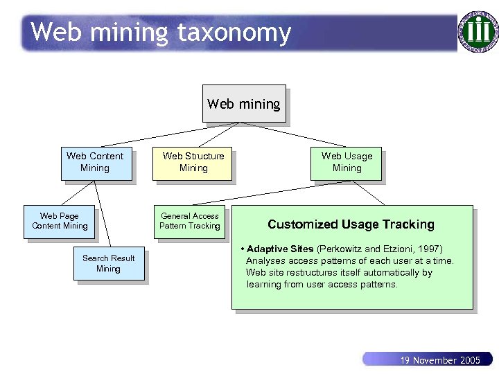Web mining taxonomy Web mining Web Content Mining Web Page Content Mining Search Result Mining Web Structure Mining General Access Pattern Tracking Web Usage Mining Customized Usage Tracking • Adaptive Sites (Perkowitz and Etzioni, 1997) Analyses access patterns of each user at a time. Web site restructures itself automatically by learning from user access patterns. 19 November 2005

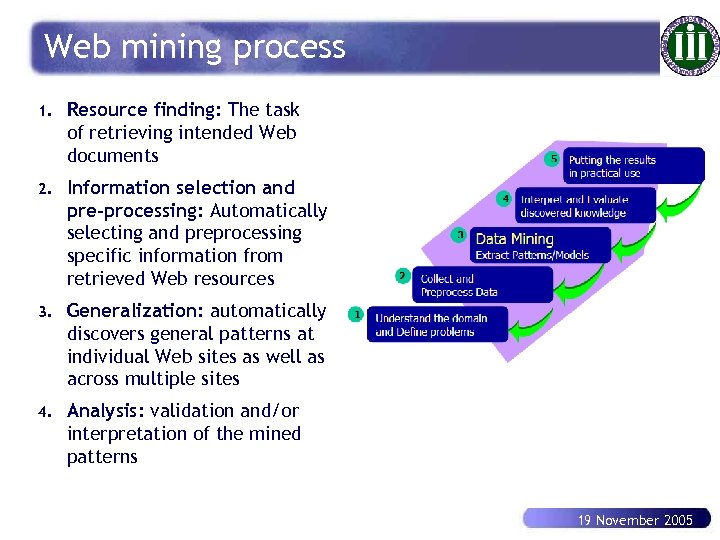Web mining process 1. Resource finding: The task of retrieving intended Web documents 2. Information selection and pre-processing: Automatically selecting and preprocessing specific information from retrieved Web resources 3. Generalization: automatically discovers general patterns at individual Web sites as well as across multiple sites 4. Analysis: validation and/or interpretation of the mined patterns 19 November 2005

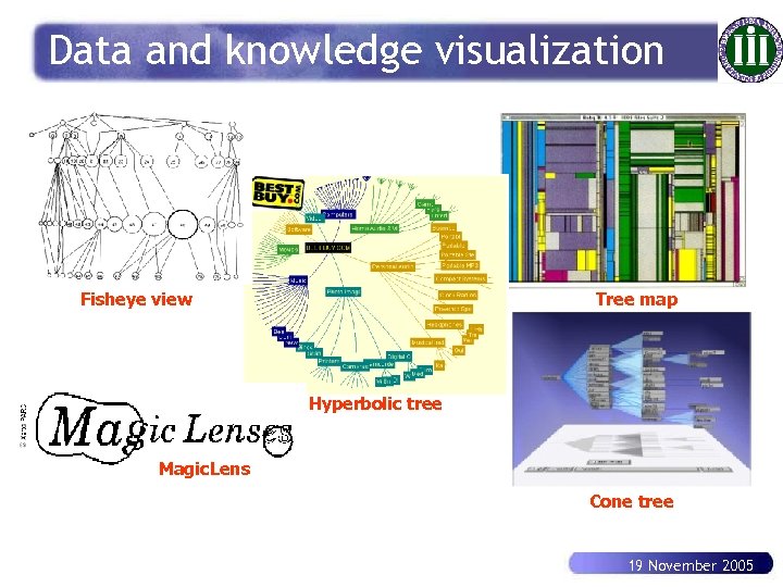Data and knowledge visualization Sunday 11 -12 PM Fisheye view Tree map Hyperbolic tree Lunch time Magic. Lens Cone tree 19 November 2005

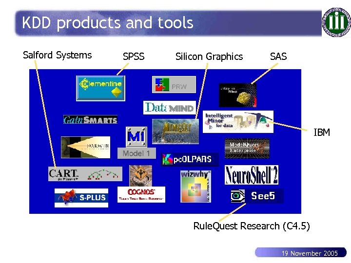KDD products and tools Salford Systems SPSS Silicon Graphics SAS IBM Rule. Quest Research (C 4. 5) 19 November 2005

Outline n Why knowledge discovery and data mining? n Basic concepts of KDD n KDD techniques: classification, association, clustering, text and Web mining n Challenges and trends in KDD n Case study in medicine data mining 19 November 2005

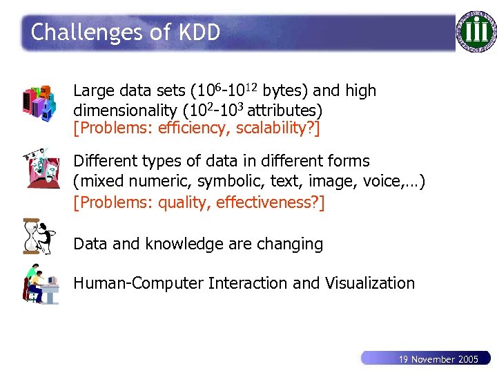Challenges of KDD Large data sets (106 -1012 bytes) and high dimensionality (102 -103 attributes) [Problems: efficiency, scalability? ] Different types of data in different forms (mixed numeric, symbolic, text, image, voice, …) [Problems: quality, effectiveness? ] Data and knowledge are changing Human-Computer Interaction and Visualization 19 November 2005

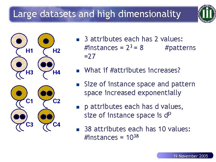Large datasets and high dimensionality n H 1 H 2 H 3 H 4 n n C 1 C 2 C 3 C 4 n n 3 attributes each has 2 values: #instances = 23 = 8 #patterns =27 What if #attributes increases? Size of instance space and pattern space increased exponentially p attributes each has d values, size of instance space is dp 38 attributes each has 10 values: #instances = 1038 19 November 2005

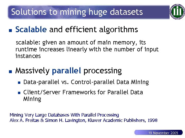
Possible solutions n Scalable and efficient algorithms (scalable: given an amount of main memory, its runtime increases linearly with the number of input instances) n Sampling (instance selection) n Dimensionality reduction (feature selection) n Approximation methods n Massively parallel processing n Integration of machine learning and database management 19 November 2005

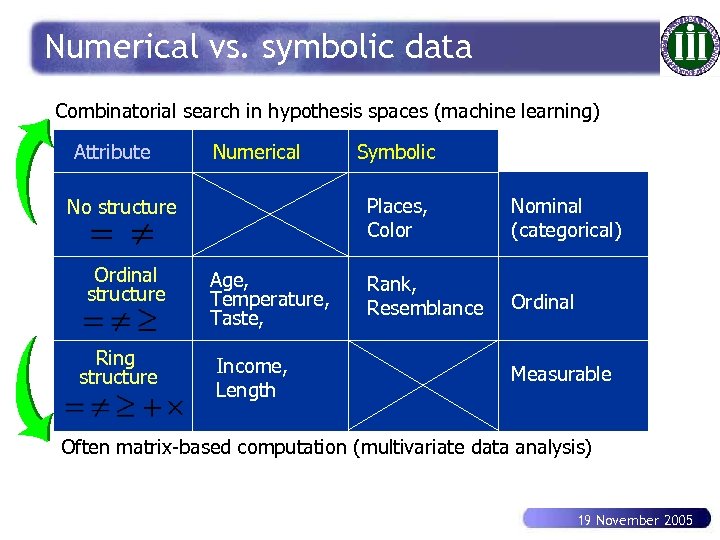Numerical vs. symbolic data Combinatorial search in hypothesis spaces (machine learning) Attribute Numerical Places, Color No structure Ordinal structure Ring structure Symbolic Age, Temperature, Taste, Income, Length Nominal (categorical) Rank, Resemblance Ordinal Measurable Often matrix-based computation (multivariate data analysis) 19 November 2005

Mining with decision trees n Attribute selection n Pruning trees n From trees to rules (high cost of pruning) n Visualization n Data access: recent development on very large training sets, fast, efficient and scalable (inmemory and secondary storage) (well-known systems: C 4. 5 and CART) 19 November 2005

Scalable decision tree induction methods n SLIQ (Mehta et al. , 1996) builds an index for each attribute and only class list and the current attribute list reside in memory n SPRINT (J. Shafer et al. , 1996) constructs an attribute list data structure n PUBLIC (Rastogi & Shim, 1998) integrates tree splitting and tree pruning: stop growing the tree earlier n Rain. Forest (Gehrke, Ramakrishnan & Ganti, 1998) è separates the scalability aspects from the criteria that determine the quality of the tree è builds an AVC-list (attribute, value, class label) 19 November 2005

Mining with neural networks n Effectively address the weakness of the symbolic AI approach in knowledge discovery (grow of the hypothesis space) n Extracting or making sense of numeric weights associated with the interconnections of neurons to come up with a higher level of knowledge has been and will continue to be a challenge problem 19 November 2005

Mining with association rules n Improving the efficiency è Database scan reduction: partitioning (Savaseve 95), hashing (Park 95), sampling (Toivonen 96), dynamic itemset counting (Brin 97), find nonredundant rules (3000 times less, Zaki KDD’ 2000) è Parallel n mining of association rules New measures of association è Interestingness è Generalized and exceptional rules and multiple-level rules 19 November 2005

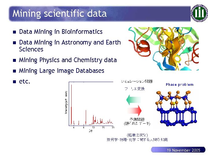Mining scientific data n Data Mining in Bioinformatics n Data Mining in Astronomy and Earth Sciences n Mining Physics and Chemistry data n Mining Large Image Databases n etc. 19 November 2005

Solutions to mining huge datasets n Scalable and efficient algorithms scalable: given an amount of main memory, its runtime increases linearly with the number of input instances n Massively parallel processing n n Data-parallel vs. Control-parallel Data Mining Client/Server Frameworks for Parallel Data Mining Very Large Databases With Parallel Processing Alex A. Freitas & Simon H. Lavington, Kluwer Academic Publishers, 1998 19 November 2005

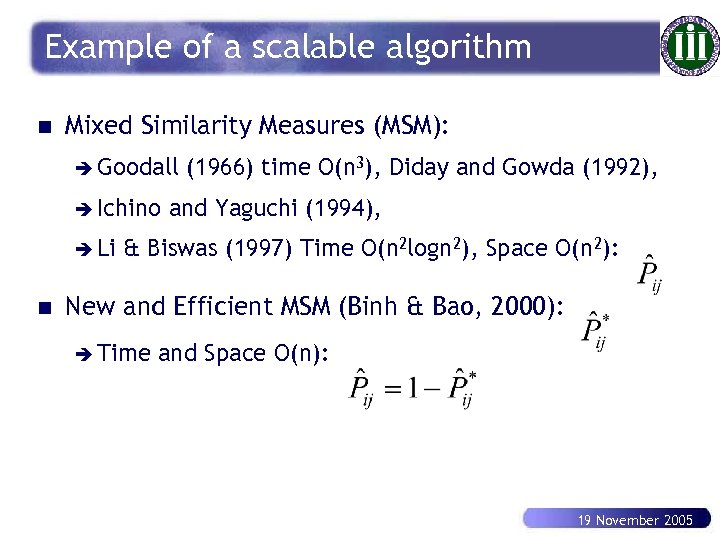Example of a scalable algorithm n Mixed Similarity Measures (MSM): è Goodall è Ichino è Li n (1966) time O(n 3), Diday and Gowda (1992), and Yaguchi (1994), & Biswas (1997) Time O(n 2 logn 2), Space O(n 2): New and Efficient MSM (Binh & Bao, 2000): è Time and Space O(n): 19 November 2005

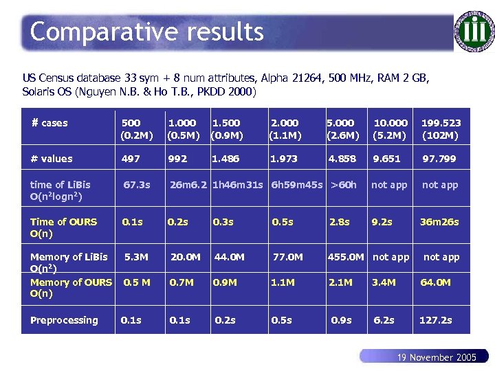Comparative results US Census database 33 sym + 8 num attributes, Alpha 21264, 500 MHz, RAM 2 GB, Solaris OS (Nguyen N. B. & Ho T. B. , PKDD 2000) ＃ cases 500 (0. 2 M) 1. 000 (0. 5 M) 1. 500 (0. 9 M) 2. 000 (1. 1 M) 5. 000 (2. 6 M) 10. 000 (5. 2 M) 199. 523 (102 M) # values 497 992 1. 486 1. 973 4. 858 9. 651 97. 799 time of Li. Bis O(n 2 logn 2) 67. 3 s 26 m 6. 2 1 h 46 m 31 s 6 h 59 m 45 s >60 h not app Time of OURS O(n) 0. 1 s 0. 2 s 9. 2 s 36 m 26 s Memory of Li. Bis O(n 2) Memory of OURS O(n) 5. 3 M Preprocessing 0. 3 s 0. 5 s 2. 8 s 20. 0 M 44. 0 M 77. 0 M 455. 0 M not app 0. 5 M 0. 7 M 0. 9 M 1. 1 M 2. 1 M 3. 4 M 64. 0 M 0. 1 s 0. 2 s 0. 5 s 0. 9 s 6. 2 s 127. 2 s 19 November 2005

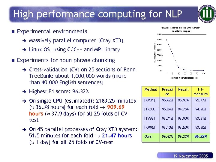High performance computing for NLP n Experimental environments è è n Massively parallel computer (Cray XT 3) Linux OS, using C/C++ and MPI library Experiments for noun phrase chunking è Cross-validation (CV) on 25 sections of Penn Tree. Bank: about 1, 000 words (more than 40, 000 English sentences) è Highest F 1 score: 96. 32% Method Precisi on Recall F 1 measure è On single CPU (estimated): 2183. 25 minutes ( 36. 38 hours) for each fold 909. 69 hours ( 37. 9 days) for all 25 folds of CVtest [KM 01] 95. 62% 95. 93% 95. 77% [TKS 00] 95. 04% 94. 75% 94. 90% [TV 99] 93. 71% 93. 90% 93. 81% On 45 parallel processes of Cray XT 3 system: 51. 5 minutes for each fold 21. 47 hours ( 1 day) for all 25 folds of CV-test [RM 95] 93. 10% 93. 50% 93. 30% Ours 96. 42% 96. 23% 96. 32% è 19 November 2005

Outline n Why knowledge discovery and data mining? n Basic concepts of KDD n KDD techniques: classification, association, clustering, text and Web mining n Challenges and trends in KDD n Case study in medicine data mining 19 November 2005

Background n HBV, HCV are viruses which both cause continuous inflammation of the liver (chronic hepatitis). n The inflammation results in liver fibrosis, and finally liver cirrhosis (LC) after 20 to 30 years which is diagnosed by liver biopsy. n In addition, the cirrhosis patients have a highly potential risk of hepatocellular carcinoma (HCC). n Physicians can treat viral hepatitis with interferon (IFN). However IFN is not always effective, with severe side effects. 19 November 2005

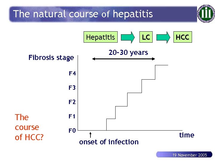The natural course of hepatitis Hepatitis Fibrosis stage LC HCC 20 -30 years F 4 F 3 F 2 The course of HCC? F 1 F 0 onset of infection time 19 November 2005

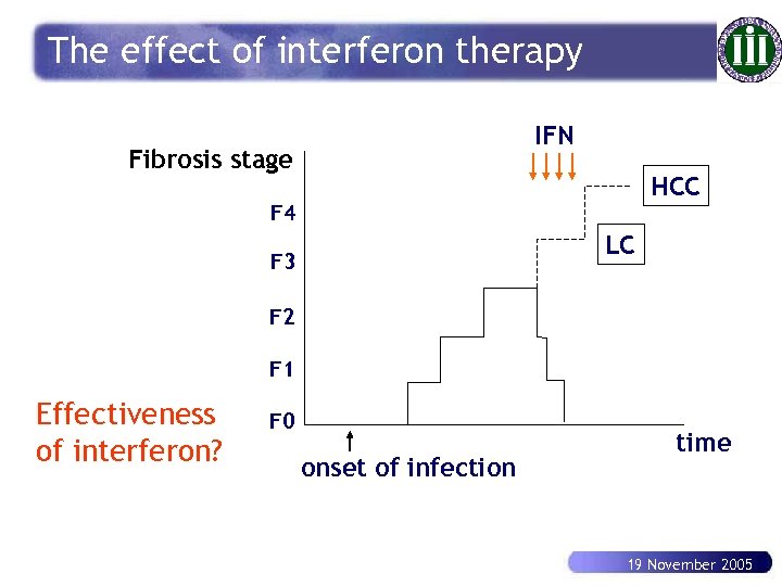The effect of interferon therapy IFN Fibrosis stage HCC F 4 LC F 3 F 2 F 1 Effectiveness of interferon? F 0 onset of infection time 19 November 2005

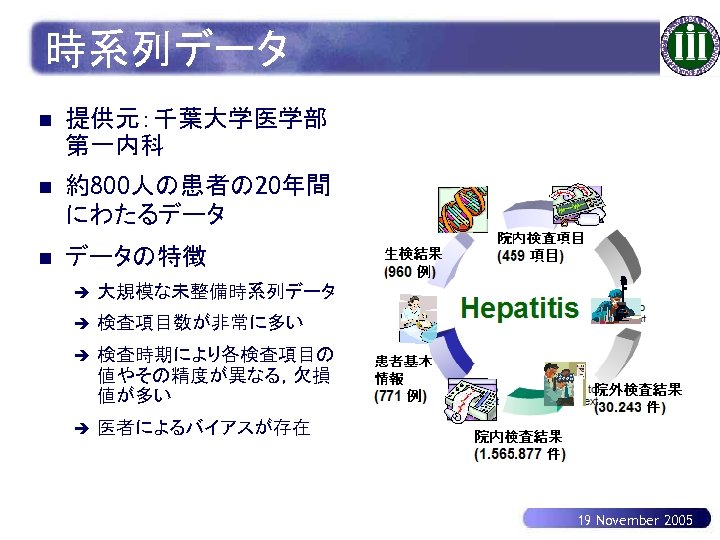時系列データ n 提供元：千葉大学医学部 第一内科 n 約800人の患者の 20年間 にわたるデータ n データの特徴 è 大規模な未整備時系列データ è 検査項目数が非常に多い è 検査時期により各検査項目の 値やその精度が異なる，欠損 値が多い è 医者によるバイアスが存在 19 November 2005

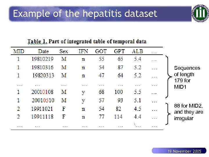Example of the hepatitis dataset Sequences of length 179 for MID 1 88 for MID 2, and they are irregular 19 November 2005

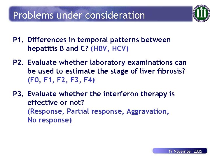Problems under consideration P 1. Differences in temporal patterns between hepatitis B and C? (HBV, HCV) P 2. Evaluate whether laboratory examinations can be used to estimate the stage of liver fibrosis? (F 0, F 1, F 2, F 3, F 4) P 3. Evaluate whether the interferon therapy is effective or not? (Response, Partial response, Aggravation, No response) 19 November 2005

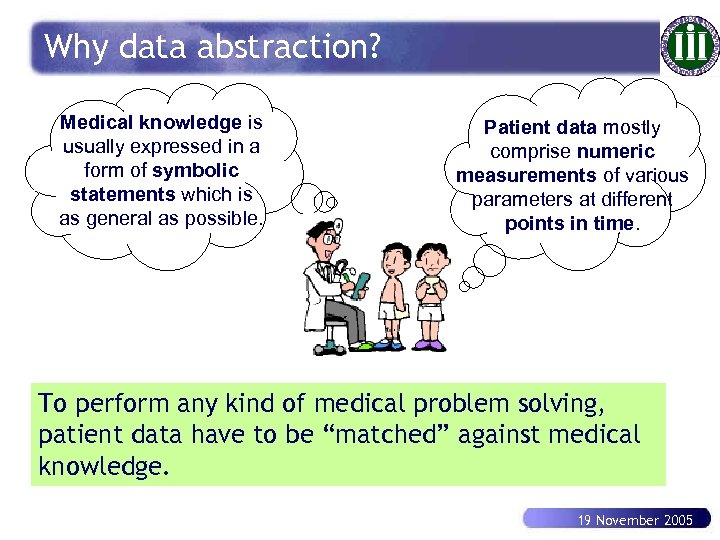Why data abstraction? Medical knowledge is usually expressed in a form of symbolic statements which is as general as possible. Patient data mostly comprise numeric measurements of various parameters at different points in time. To perform any kind of medical problem solving, patient data have to be “matched” against medical knowledge. 19 November 2005

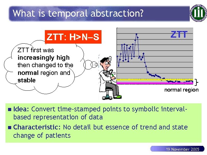What is temporal abstraction? ZTT: H>N S ZTT first was increasingly high then changed to the normal region and stable normal region n Idea: Convert time-stamped points to symbolic intervalbased representation of data n Characteristic: No detail but essence of trend and state change of patients 19 November 2005

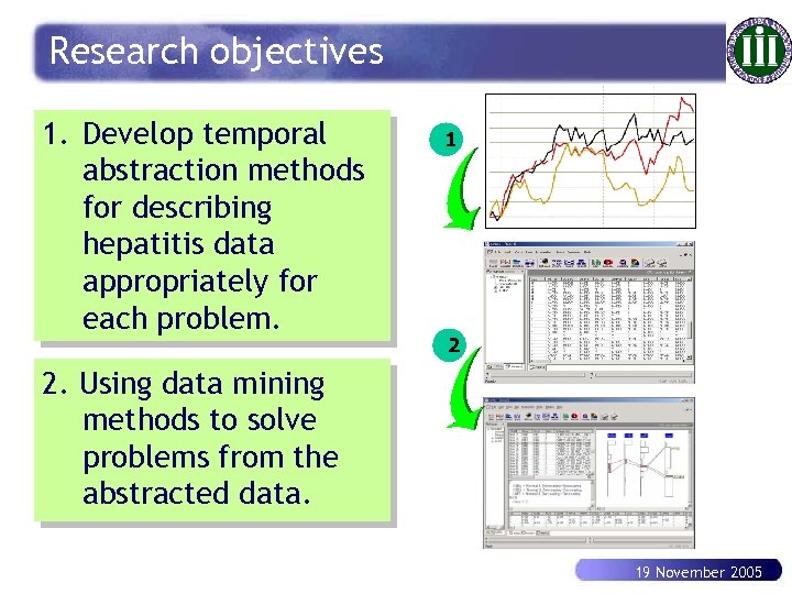Research objectives 1. Develop temporal abstraction methods for describing hepatitis data appropriately for each problem. 1 2 2. Using data mining methods to solve problems from the abstracted data. 19 November 2005

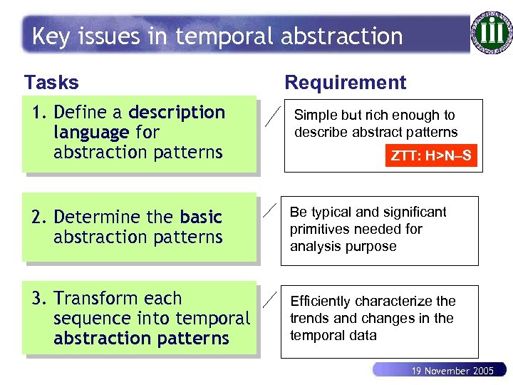Key issues in temporal abstraction Tasks Requirement 1. Define a description language for abstraction patterns Simple but rich enough to describe abstract patterns 2. Determine the basic abstraction patterns Be typical and significant primitives needed for analysis purpose 3. Transform each sequence into temporal abstraction patterns Efficiently characterize the trends and changes in the temporal data ZTT: H>N S 19 November 2005

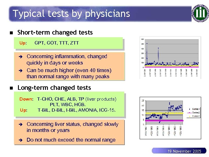Typical tests by physicians n Short-term changed tests Up: è è n GPT, GOT, TTT, ZTT Concerning inflammation, changed quickly in days or weeks Can be much higher (even 40 times) than normal range with many peaks Long-term changed tests Down: T-CHO, CHE, ALB, TP (liver products) PLT, WBC, HGB. Up: T-BIL, D-BIL, I-BIL, AMONIA, ICG-15. è Concerning liver status, changed slowly in months or years è Do not much exceed the normal range 19 November 2005

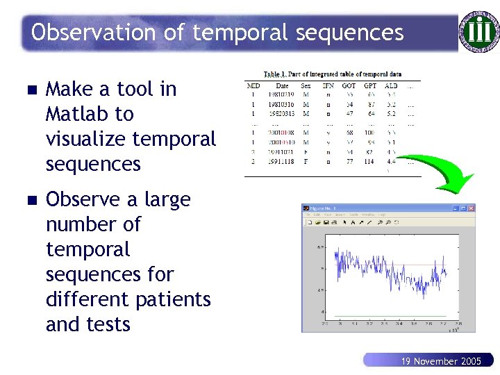Observation of temporal sequences n Make a tool in Matlab to visualize temporal sequences n Observe a large number of temporal sequences for different patients and tests 19 November 2005

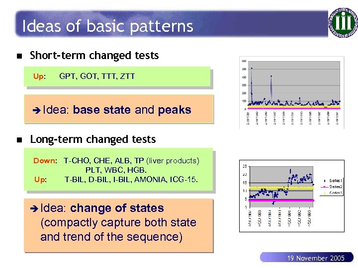Ideas of basic patterns n Short-term changed tests Up: GPT, GOT, TTT, ZTT è Idea: n base state and peaks Long-term changed tests Down: T-CHO, CHE, ALB, TP (liver products) PLT, WBC, HGB. Up: T-BIL, D-BIL, I-BIL, AMONIA, ICG-15. è Idea: change of states (compactly capture both state and trend of the sequence) 19 November 2005

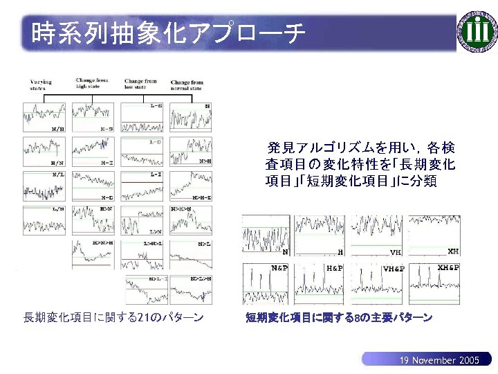時系列抽象化アプローチ 　　発見アルゴリズムを用い，各検 査項目の変化特性を「長期変化 項目」「短期変化項目」に分類 長期変化項目に関する21のパターン 短期変化項目に関する8の主要パターン 19 November 2005

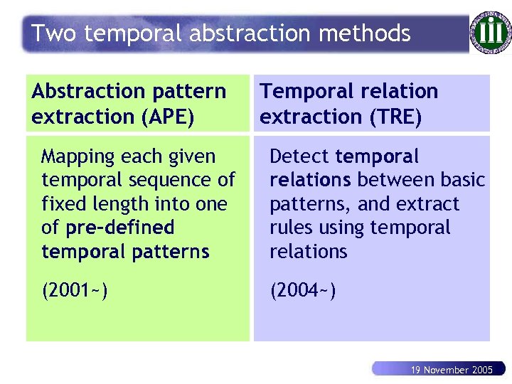Two temporal abstraction methods Abstraction pattern extraction (APE) Temporal relation extraction (TRE) Mapping each given temporal sequence of fixed length into one of pre-defined temporal patterns Detect temporal relations between basic patterns, and extract rules using temporal relations (2001~) (2004~) 19 November 2005

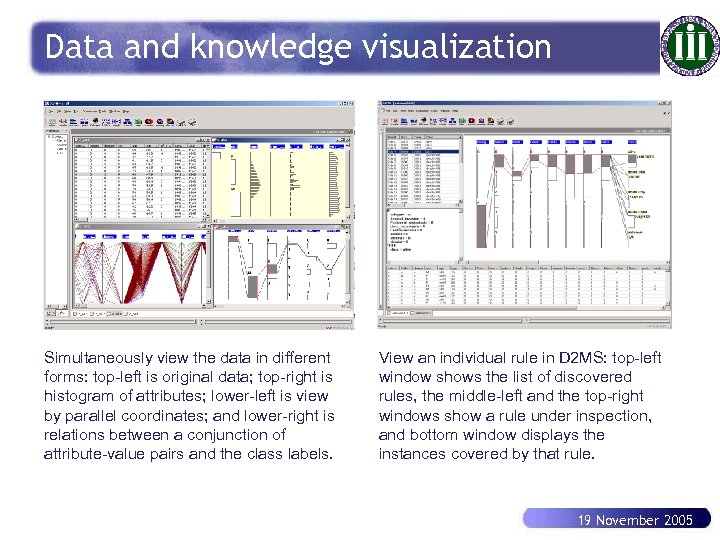Data and knowledge visualization Simultaneously view the data in different forms: top-left is original data; top-right is histogram of attributes; lower-left is view by parallel coordinates; and lower-right is relations between a conjunction of attribute-value pairs and the class labels. View an individual rule in D 2 MS: top-left window shows the list of discovered rules, the middle-left and the top-right windows show a rule under inspection, and bottom window displays the instances covered by that rule. 19 November 2005

LC vs. non-LC 19 November 2005

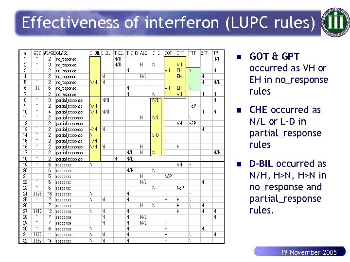Effectiveness of interferon (LUPC rules) n GOT & GPT occurred as VH or EH in no_response rules n CHE occurred as N/L or L-D in partial_response rules n D-BIL occurred as N/H, H>N in no_response and partial_response rules. 19 November 2005

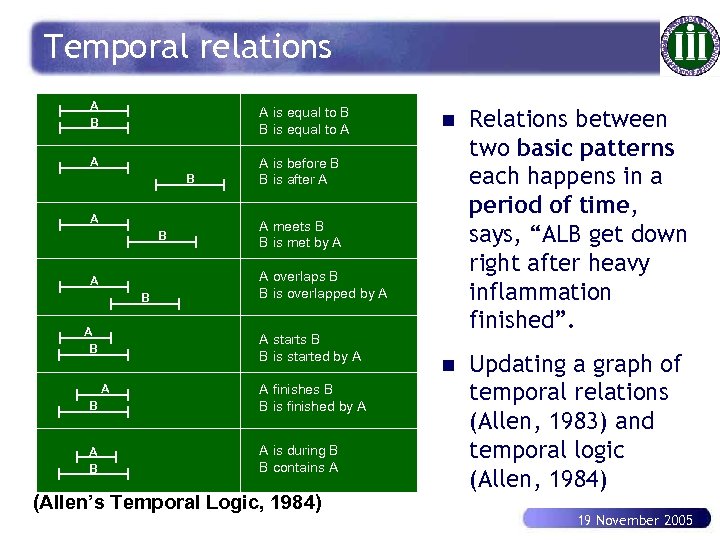Temporal relations A B A is equal to B B is equal to A A A is before B B is after A B A B Relations between two basic patterns each happens in a period of time, says, “ALB get down right after heavy inflammation finished”. n Updating a graph of temporal relations (Allen, 1983) and temporal logic (Allen, 1984) A meets B B is met by A A overlaps B B is overlapped by A A starts B B is started by A B A finishes B B is finished by A A B A is during B B contains A A n (Allen’s Temporal Logic, 1984) 19 November 2005

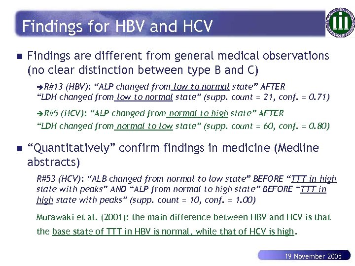Findings for HBV and HCV n Findings are different from general medical observations (no clear distinction between type B and C) èR#13 (HBV): “ALP changed from low to normal state” AFTER “LDH changed from low to normal state” (supp. count = 21, conf. = 0. 71) èR#5 (HCV): “ALP changed from normal to high state” AFTER “LDH changed from normal to low state” (supp. count = 60, conf. = 0. 80) n “Quantitatively” confirm findings in medicine (Medline abstracts) R#53 (HCV): “ALB changed from normal to low state” BEFORE “TTT in high state with peaks” AND “ALP from normal to high state” BEFORE “TTT in high state with peaks” (supp. count = 10, conf. = 1. 00) Murawaki et al. (2001): the main difference between HBV and HCV is that the base state of TTT in HBV is normal, while that of HCV is high. 19 November 2005

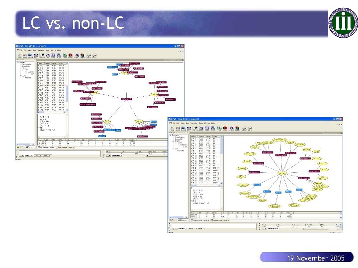
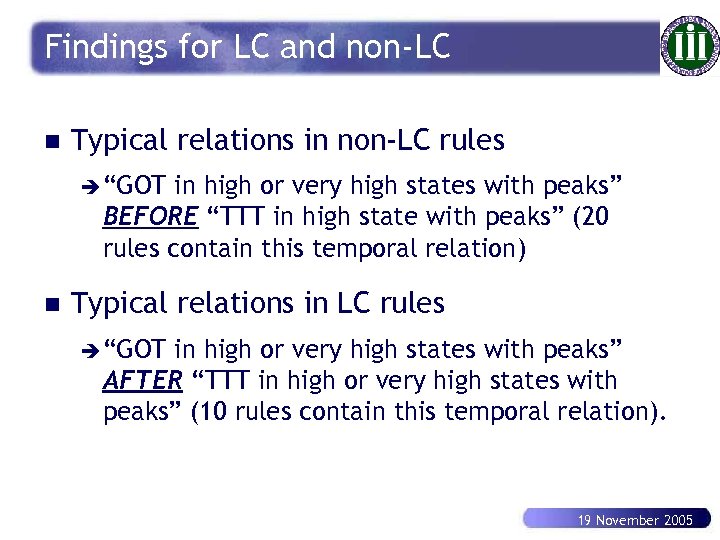Findings for LC and non-LC n Typical relations in non-LC rules è “GOT in high or very high states with peaks” BEFORE “TTT in high state with peaks” (20 rules contain this temporal relation) n Typical relations in LC rules è “GOT in high or very high states with peaks” AFTER “TTT in high or very high states with peaks” (10 rules contain this temporal relation). 19 November 2005

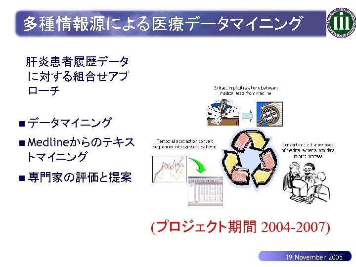多種情報源による医療データマイニング 肝炎患者履歴データ に対する組合せアプ ローチ n データマイニング n Medlineからのテキス トマイニング n 専門家の評価と提案 (プロジェクト期間 2004 -2007) 19 November 2005

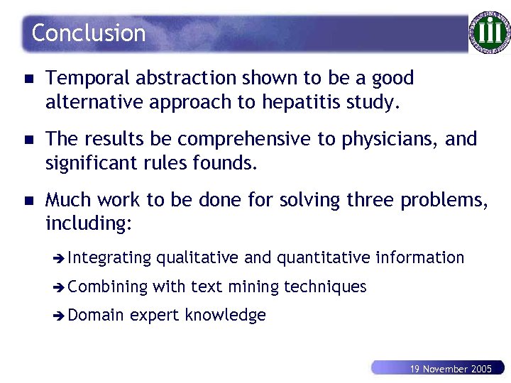Conclusion n Temporal abstraction shown to be a good alternative approach to hepatitis study. n The results be comprehensive to physicians, and significant rules founds. n Much work to be done for solving three problems, including: è Integrating qualitative and quantitative information è Combining with text mining techniques è Domain expert knowledge 19 November 2005

Summary n KDD is motivated by the wide availability of huge amounts of data and the imminent need for turning such data into useful information and knowledge. n There are different methods to find predictive or descriptive models that strongly depend on the data schemes. n The KDD process is necessarily interactive and iterative, and requires human participation in all steps of the process. 19 November 2005

Recommended references n http: //www. kdnuggets. com n David J. Hand, Heikki Mannila and Padhraic Smyth, Principles of Data Mining, MIT Press, 2000 n Jiawei Han, Micheline Kamber, Data Mining : Concepts and Techniques, Morgan Kaufmann, 2000 n U. Fayyad, G. Piatetsky-Shapiro, P. Smyth, R. Uthurusamy, editors, Advances in Knowledge Discovery and Data Mining, AAAI/MIT Press, 1996. 19 November 2005

Acknowledgments n Profs. S. Ohsuga, M. Kimura, H. Motoda, H. Shimodaira, Y. Nakamori, S. Horiguchi, T. Mitani, T. Tsuji, K. Satou, among others n Nguyen N. B. , Nguyen T. D. , Kawasaki S. , Huynh V. N. , Dam H. C. , Tran T. N. , Pham T. H. , Nguyen D. D. , Nguyen L. M. , Phan X. H. , Le M. H. , Hassine B. A. , Le S. Q. , Zhang H. , Nguyen C. H. , Nagai K. , Nguyen C. H. , Nguyen T. P. , Tran D. H. 19 November 2005