bc1539c603c5b6e908014952e6b908a0.ppt
- Количество слайдов: 111
 Introduction to Fuzzy Logic Adnan Yazici Dept. of Computer Engineering, Middle East Technical University, 06531, Ankara/Turkey
 Introduction Ø “Mathematics that refers to reality is not certain and mathematics that is certain does not refer to reality” Albert Einstein Ø “While the mathematician constructs a theory in terms of ´perfect´objects, the experimental observes objects of which the properties demanded by theory are and can, in the very nature of measurement, be only approximately true” Max Black Ø “What makes society turn is science, and the language of science is math, and the structure of math is logic, and the bedrock of logic is Aristotle, and that is what goes out with fuzzy logic” Bart Kosko
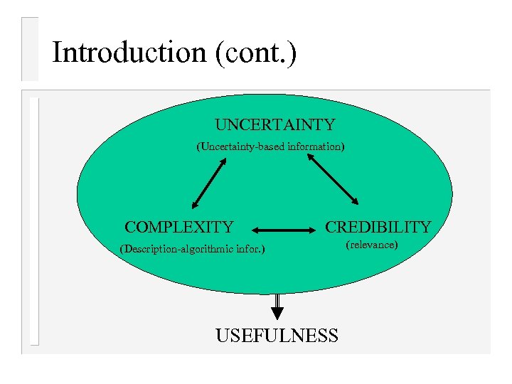
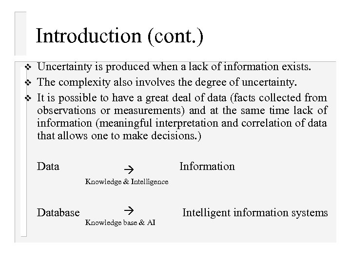 Introduction (cont. ) v v v Uncertainty is produced when a lack of information exists. The complexity also involves the degree of uncertainty. It is possible to have a great deal of data (facts collected from observations or measurements) and at the same time lack of information (meaningful interpretation and correlation of data that allows one to make decisions. ) Data Information Knowledge & Intelligence Database Intelligent information systems Knowledge base & AI
 Introduction (cont. ) Knowledge is information at a higher level of abstraction. Ex: Ali is 10 years old (fact) Ali is not old (knowledge) Ø Our problems are: v v v Ø Solutions are: v v v Ø Ø Decision Management Prediction Faster access to more information and of increased aid in analysis Understanding – utilizing information available Managing with information not avaliable Large amount of information with large amount of uncertainty lead to complexity. Avareness of knowledge (what we know and what we do not know) and complexity goes together. Ex: Driving a car is complex, driving in an iced road is more compex, since more knowledge is needed for driving in an iced road.
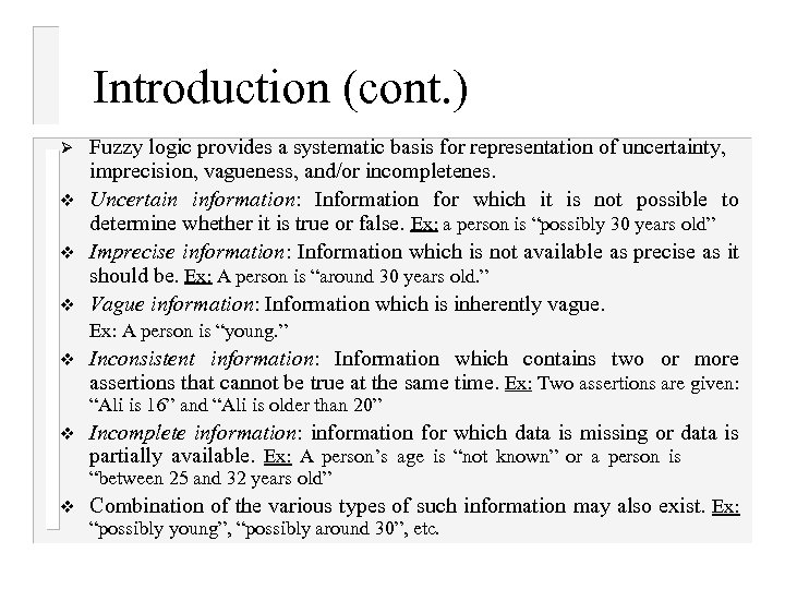 Introduction (cont. ) Ø v v v Fuzzy logic provides a systematic basis for representation of uncertainty, imprecision, vagueness, and/or incompletenes. Uncertain information: Information for which it is not possible to determine whether it is true or false. Ex: a person is “possibly 30 years old” Imprecise information: Information which is not available as precise as it should be. Ex: A person is “around 30 years old. ” Vague information: Information which is inherently vague. Ex: A person is “young. ” v Inconsistent information: Information which contains two or more assertions that cannot be true at the same time. Ex: Two assertions are given: “Ali is 16” and “Ali is older than 20” v Incomplete information: information for which data is missing or data is partially available. Ex: A person’s age is “not known” or a person is “between 25 and 32 years old” v Combination of the various types of such information may also exist. Ex: “possibly young”, “possibly around 30”, etc.
 Introduction (cont. ) UNCERTAINTY (Uncertainty-based information) COMPLEXITY CREDIBILITY (Description-algorithmic infor. ) USEFULNESS (relevance)
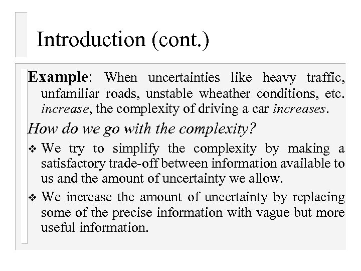 Introduction (cont. ) Example: When uncertainties like heavy traffic, unfamiliar roads, unstable wheather conditions, etc. increase, the complexity of driving a car increases. How do we go with the complexity? We try to simplify the complexity by making a satisfactory trade-off between information available to us and the amount of uncertainty we allow. v We increase the amount of uncertainty by replacing some of the precise information with vague but more useful information. v
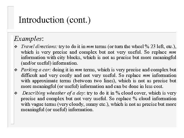 Introduction (cont. ) Examples: v v v Travel directions: try to do it in mm terms (or turn the wheel % 23 left, etc. ), which is very precise and complex but not very useful. So replace mm information with city blocks, which is not as precise but more meaningful (and/or useful) information. Parking a car: doing it in mm terms, which is very precise and complex but difficult and very costly and not very useful. So replace mm information with approximate terms (between two lines), which is not as precise but more meaningful (or useful) information and can be done in less cost. Describing wheather of a day: try to do it in % cloud cover, which is very precise and complex but not very useful. So replace % cloud information with vague terms (very cloudy, sunny etc. ), which is not as precise but more meaningful (or useful) information.
 Introduction (cont. ) Ø v v Fuzzy logic has been used for two different senses: In a narrow sense: refers to logical system generalizing crisp logic for reasoning uncertainty. In a broad sense: refers to all of theories and technologies that employ fuzzy sets, which are classes with imprecise boundaries. The broad sense of fuzzy logic includes the narrow sense of fuzzy logic as a branch. Other areas include fuzzy control, fuzzy pattern recongnition, fuzzy arithmetic, fuzzy probability theory, fuzzy decision analysis, fuzzy databases, fuzzy expert systems, fuzzy computer SW and HW, etc.
 Introduction (cont. ) With Fuzzy Logic, one can accomplish two things: v Ease of describing human knowledge involving vague concepts v Enhanced ability to develop a cost-effective solution to realworld Ø In another word, fuzzy logic not only provides a cost effective way to model complex systems involving numeric variables but also offers a quantitative description of the system that is easy to comprehend.
 Introduction (cont. ) Fuzzy Logic was motivated by two objectives: v First, it aims to alleviate difficulties in developing and analyzing complex systems encountered by conventional mathematical tools. This motivation requires fuzzy logic to work in quantitative and numeric domains. v Second, it is motivated by observing that human reasoning can utilize concepts and knowledge that do not have well defined, sharp boundaries (i. e. , vague concepts). This motivation enables fuzzy logic to have a descriptive and qualitative form. This is related to AI.
 Introduction (cont. ) Components of Fuzzy Logic v Fuzzy Predicates: tall, small, kind, expensive, . . . v Predicates modifiers (hedges): very, quite, more or less, extremely, . . v Fuzzy truth values: true, very true, fairly false, . . . v Fuzzy quantifiers: most, few, almost, usually, . . v Fuzzy probabilities: likely, very likely, highly likely, . . .
 Introduction (cont. ) Applications v Control: “If the temperature is very high and the presure is decreasing rapidly, then reduce the heat significantly. ” v Database: “Retrieve the names of all candidates that are fairly young, have a strong background in algorithms, and a modest administrative experience. ” v Medicine: Hepatitis is characterized by the statement, ‘Total proteins are usually normal, albumin is decreased, -globulins are slightly decreased, globulins are increased’
 Introduction (cont. ) Ø Probability theory vs fuzzy set theory: v Probability measures the likelihood of a future event, based on something known now. Probability is theory of random events and is not capable of capturing uncertainty resulting from vagueness of linguistic terms. v Fuzziness is not the uncertainty of expectation. It is the uncertainty resulting from imprecision of meaning of a concept expressed by a linguistic term in NL, such as “tall” or “warm” etc.
 Introduction (cont. ) Ø Probability theory vs fuzzy set theory (cont): v Fuzzy set theory makes statements about one concrete object; therefore, modeling local vagueness, whereas probability theory makes statements about a collection of objects from which one is selected; therefore, modeling global uncertainty. Fuzzy logic and probability complement each other. Example: “highly probable” is a concept that involves both randomness and fuziness. The behaviour of a fuzzy system is completely deterministic. Fuzzy logic differs from multivalued logic by introducing concepts such as linguistic variables and hedges to capture human linguistic reasoning. v v v
 Introduction (cont. ) Ø v v ü Even though the broad sense of fuzzy logic covers a wide range of theories and techniques, its core technique is based on four basic concepts: Fuzzy sets: sets with smooth boundaries; Linguistic variables: variables whose values are both qualitatively and quantitatively described by a fuzzy set; Possibility distribution: constraints on the value of a linguistic variable imposed by assigning it a fuzzy set; and Fuzzy if-then rules: a knowledge representation scheme for describing a functional mapping (fuzzy mapping rules) or a logical formula that generalizes an implication in two-valued logic (fuzzy implication rules). The first three concepts are fundamental for all subareas in fuzzy logic, but the fourth one is also important.
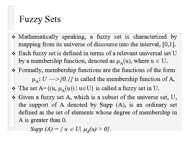 Fuzzy Sets v v v Mathematically speaking, a fuzzy set is characterized by mapping from its universe of discourse into the interval, [0, 1]. Each fuzzy set is defined in terms of a relevant universal set U by a membership function, denoted as A(u), where u U. Formally, membership functions are the functions of the form A: U --> [0, 1] is called the membership function of A. The set A={(u, A(u)) | u U} is called a fuzzy set in U. Given a fuzzy set A, which is a subset of the universe set, U, the support of A denoted by Supp (A), is an ordinary set defined as the set of elements whose degree of membership in A is greater than 0. Supp (A) = { u U| A(u) > 0}.
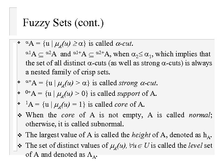 Fuzzy Sets (cont. ) v A = {u | A(u) } is called -cut. 1 A 2 A and 1+A 2+A, when v v v 2 1, which implies that the set of all distinct -cuts (as well as strong -cuts) is always a nested family of crisp sets. +A = {u | (u) > } is called strong -cut. A 0+A = {u | (u) > 0} is called support of A. A 1 A = {u | (u) = 1} is called core of A. A When the core of A is not empty, A is called normal; otherwise, it is called subnormal. The largest value of A is called the height of A, denoted as h. A. The set of distinct values of A(u), u U is called the level set of A and denoted as A.
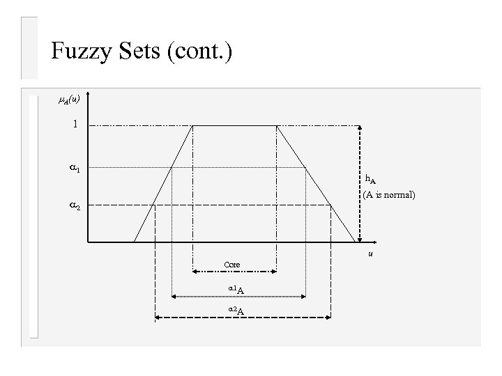 Fuzzy Sets (cont. ) A(u) 1 1 h. A (A is normal) 2 u Core 1 A 2 A
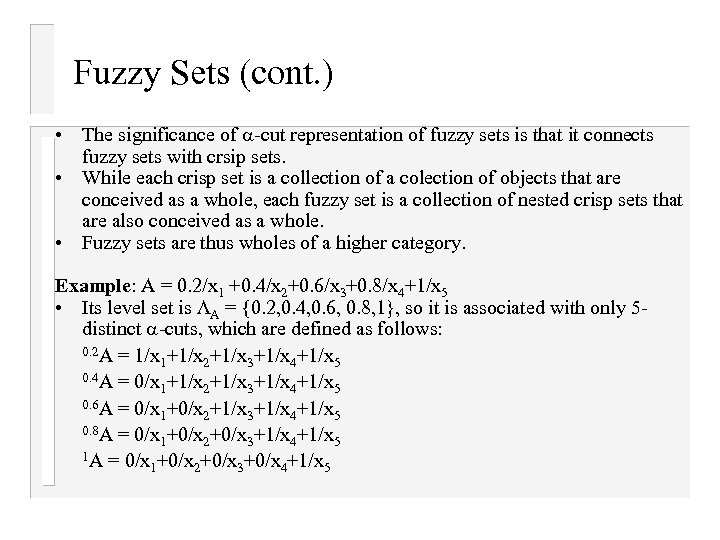 Fuzzy Sets (cont. ) • The significance of -cut representation of fuzzy sets is that it connects fuzzy sets with crsip sets. • While each crisp set is a collection of a colection of objects that are conceived as a whole, each fuzzy set is a collection of nested crisp sets that are also conceived as a whole. • Fuzzy sets are thus wholes of a higher category. Example: A = 0. 2/x 1 +0. 4/x 2+0. 6/x 3+0. 8/x 4+1/x 5 • Its level set is A = {0. 2, 0. 4, 0. 6, 0. 8, 1}, so it is associated with only 5 distinct -cuts, which are defined as follows: 0. 2 A = 1/x +1/x 1 2 3 4 5 0. 4 A = 0/x +1/x 1 2 3 4 5 0. 6 A = 0/x +1/x 1 2 3 4 5 0. 8 A = 0/x +0/x +1/x 1 2 3 4 5 1 A = 0/x +0/x +1/x 1 2 3 4 5
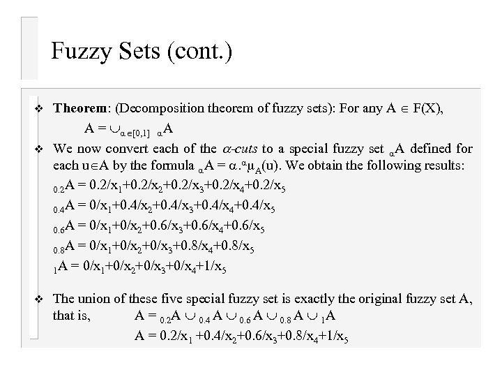 Fuzzy Sets (cont. ) v v v Theorem: (Decomposition theorem of fuzzy sets): For any A F(X), A = [0, 1] A We now convert each of the -cuts to a special fuzzy set A defined for each u A by the formula A = . A(u). We obtain the following results: 0. 2 A = 0. 2/x 1+0. 2/x 2+0. 2/x 3+0. 2/x 4+0. 2/x 5 0. 4 A = 0/x 1+0. 4/x 2+0. 4/x 3+0. 4/x 4+0. 4/x 5 0. 6 A = 0/x 1+0/x 2+0. 6/x 3+0. 6/x 4+0. 6/x 5 0. 8 A = 0/x 1+0/x 2+0/x 3+0. 8/x 4+0. 8/x 5 1 A = 0/x 1+0/x 2+0/x 3+0/x 4+1/x 5 The union of these five special fuzzy set is exactly the original fuzzy set A, that is, A = 0. 2 A 0. 4 A 0. 6 A 0. 8 A 1 A A = 0. 2/x 1 +0. 4/x 2+0. 6/x 3+0. 8/x 4+1/x 5
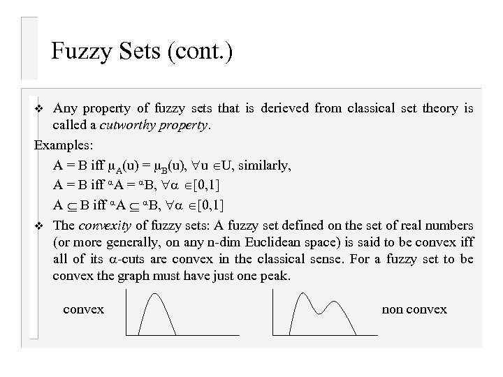 Fuzzy Sets (cont. ) Any property of fuzzy sets that is derieved from classical set theory is called a cutworthy property. Examples: A = B iff A(u) = B(u), u U, similarly, A = B iff A = B, [0, 1] A B iff A B, [0, 1] v The convexity of fuzzy sets: A fuzzy set defined on the set of real numbers (or more generally, on any n-dim Euclidean space) is said to be convex iff all of its -cuts are convex in the classical sense. For a fuzzy set to be convex the graph must have just one peak. v convex non convex
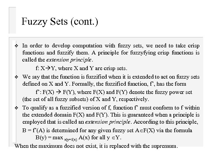 Fuzzy Sets (cont. ) In order to develop computation with fuzzy sets, we need to take crisp functions and fuzzify them. A principle for fuzzyfying crisp functions is called the extension principle. f: X Y, where X and Y are crisp sets. v We say that the function is fuzzified when it is extended to act on fuzzy sets defined on X and Y. Formally, the fuzzified function, f’, has the form f’: F(X) F(Y), where F(X) and F(Y) denote the fuzzy power set (the set of all fuzzy subsets) of X and Y, respectively. v To qualify as a fuzzified version of f, function f’ must conform to f within the extended domain F(X) and F(Y). This is guaranteed when a principle is employed that is called an extension principle. According to this principle, B = f’(A) is determined for any given fuzzy set A F(X) via the formula B(y) = max x|y=f(x) A(x) for all y Y. When the maximum does not exist, it is replaced with the supremum. v
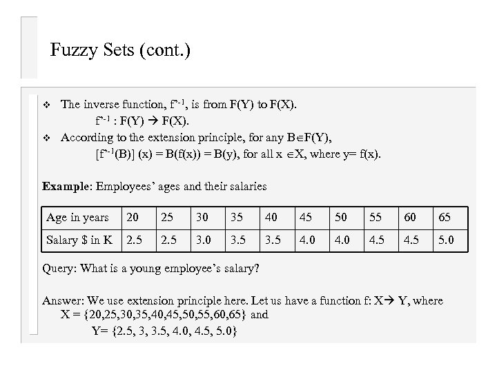 Fuzzy Sets (cont. ) v v The inverse function, f’-1, is from F(Y) to F(X). f’-1 : F(Y) F(X). According to the extension principle, for any B F(Y), [f’-1(B)] (x) = B(f(x)) = B(y), for all x X, where y= f(x). Example: Employees’ ages and their salaries Age in years 20 25 30 35 40 45 50 55 60 65 Salary $ in K 2. 5 3. 0 3. 5 4. 0 4. 5 5. 0 Query: What is a young employee’s salary? Answer: We use extension principle here. Let us have a function f: X Y, where X = {20, 25, 30, 35, 40, 45, 50, 55, 60, 65} and Y= {2. 5, 3, 3. 5, 4. 0, 4. 5, 5. 0}
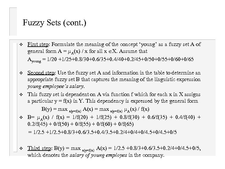 Fuzzy Sets (cont. ) v First step: Formulate the meaning of the concept ‘young’ as a fuzzy set A of general form A = A(x) / x for all x X. Assume that Ayoung = 1/20 +1/25+0. 8/30+0. 6/35+0. 4/40+0. 2/45+0/50+0/55+0/60+0/65 v Second step: Use the fuzzy set A and information in the table to determine an appropriate fuzzy set B that captures the meaning of the linguistic expression young employee’s salary. This fuzzy set is dependent on A via function f which for each x in X assigns a particular y = f(x) in Y. This dependency is expressed by the general form B(y) = max x|y=f(x) A(x) / f(x) B= A(x) / f(x) = 1/f(20) + 1/f(25) + 0. 8/f(30) + 0. 6/f(35) + 0. 4/f(40) + 0. 2/f(45) + 0/f(50) + 0/f(55) + 0/f(60) + 0/f(65) = 1/2. 5 +1/2. 5+0. 8/3+0. 6/3. 5+0. 4/3. 5+0. 2/4+0/4. 5+0/5 v v v Third step: B(y) = max x|y=f(x) A(x) = 1/2. 5 +0. 8/3+0. 6/3. 5+0. 2/4+0/4. 5+0/5, which denotes the salary of young employes in the company.
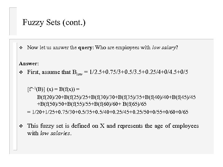 Fuzzy Sets (cont. ) v Now let us answer the query: Who are employees with low salary? Answer: v First, assume that Blow = 1/2. 5+0. 75/3+0. 5/3. 5+0. 25/4+0/4. 5+0/5 [f’-1(B)] (x) = B(f(x)) = B(f(20)/20+B(f(25)/25+B(f(30)/30+B(f(35)/35+B(f(40)/40+B(f(45)/45 +B(f(50)/50+B(f(55)/55+B(f(60)/60+ B(f(65)/65 = 1/20+1/25+0. 75/30+0. 5/35+0. 5/40+0. 25/45+0. 25/50+0/55+0/60+0/65 v This fuzzy set is defined on X and represents the age of employees with low salaries.
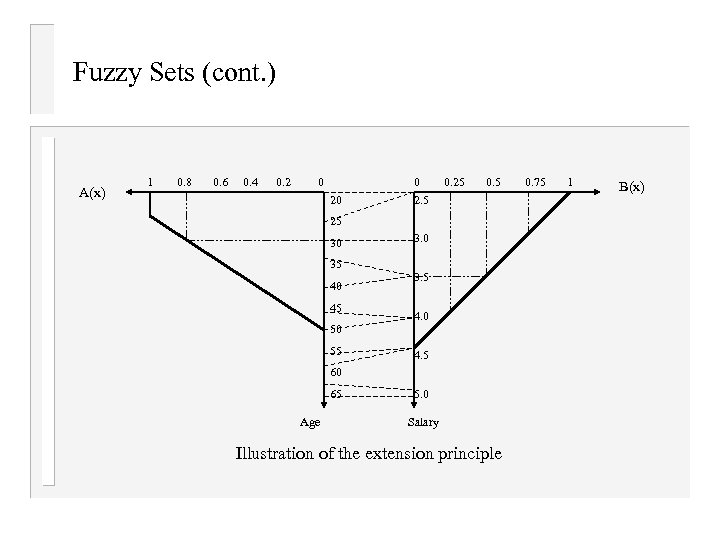 Fuzzy Sets (cont. ) A(x) 1 0. 8 0. 6 0. 4 0. 2 0 20 0 0. 25 0. 75 1 2. 5 25 30 35 40 45 50 55 3. 0 3. 5 4. 0 4. 5 60 65 Age 5. 0 Salary Illustration of the extension principle B(x)
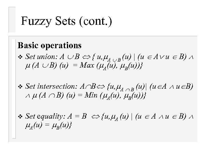 Fuzzy Sets (cont. ) Basic operations v Set union: A B { u, A B (u) | (u A u B) (A B) (u) = Max ( A(u), B(u))} v Set intersection: A B {u, A B (u)| (u A u B) (A B) (u) = Min ( A(u), B(u))} v Set equality: A = B {u, A (u) | (u A u B) A(u) = B(u)}
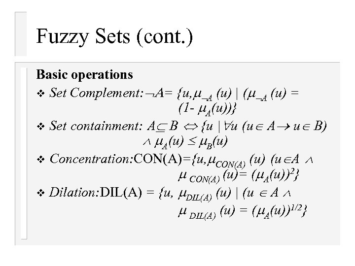 Fuzzy Sets (cont. ) Basic operations v Set Complement: = {u, A (u) | ( A (u) = (1 - A(u))} v Set containment: A B {u | u (u A u B) A(u) B(u) v Concentration: CON(A)={u, CON(A) (u A CON(A) (u)= ( A(u))2} v Dilation: DIL(A) = {u, DIL(A) (u) | (u A DIL(A) (u) = ( A(u))1/2}
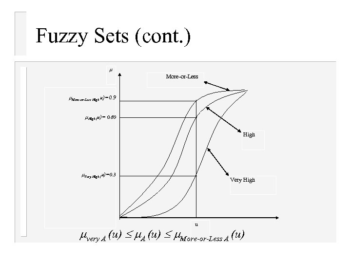 Fuzzy Sets (cont. ) More-or-Less High u)=0. 9 High (u)= 0. 80 High Very High (u)=0. 3 Very High u very A (u) More-or-Less A (u)
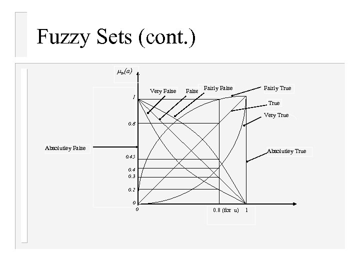 Fuzzy Sets (cont. ) tv(a) Very False 1 False Fairly False Fairly True Very True 0. 8 Absolutley False Absolutley True 0. 45 0. 4 0. 3 0. 2 0 0 0. 8 (for u) 1
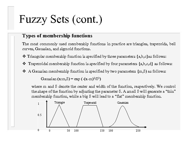 Fuzzy Sets (cont. ) Types of membership functions The most commonly used membership functions in practice are triangles, trapezoids, bell curves, Gaussian, and sigmoid functions. v Triangular membership function is specified by three parameters {a, b, c}as follows: v Trapezoidal membership function is specified by four parameters {a, b, c, d} as follows: v A Gaussian membership function is specified by two parameters {m, ) as follows: Gaussian (x: m, ) = exp (-(x-m)2/ 2) where m and denote the center and width of the function, respectively. We control the shape of the function by adjusting the parameter . A small will generate a “thin” membership function, while a big will lead to a “flat” membership function. 1 Triangle Trapezoid Gaussian 0. 5 0 0 50 100 150 100 250
 Fuzzy Sets (cont. ) Designing membership functions How do we determine the exact shape of the membership function for a fuzzy set? A membership function can be designed in three ways: v Interview those who are familiar with the underlying concepts and later adjust it based on a tuning strategy, v Construct it automatically from data, v Learn it based on feedback from the system performance.
 Fuzzy Sets (cont. ) The guidelines for membership function design v Use parameterizable functions that can be defined by a small number of parameters. Parameterizable membership functions reduce the system design time and facilitate the automated tuning of the system. v The parameterizable membership functions most commonly used in practice are the triangular and trapezoidal membership functions, because of their simplicity. v If you want to learn the membership function using neural network learning techniques, choose a differentiable (or even continuous differentiable) membership function (e. g. , Gaussian).
 Fuzzy Sets (cont. ) v v v Designing antecedent membership functions The membership functions of an input variable’s fuzzy sets should usually be designed in a way that the following two conditions are satisfied: Unless there is a good reason, use symmetric membership functions. This guideline has an additional benefit from the viewpoint of stability analysis. Each membership function overlaps only with the closest neighboring membership functions; Ai Aj = j i, j+1, i-1, where Ai are fuzzy sets. For any possible input data, its membership values in all relevant fuzzy sets should sum to 1 (or nearly so), i Ai (x) 1
 Linguistic Variables Ø Ø A linguistic variable enables its value to be described both qualitatively by a linguistic term (i. e. , a symbol serving as the name of a fuzzy set) and quantitatively by a corresponding membership function, (which express the meaning of the fuzzy set). For example, if Trading. Quantity is Heavy, the fuzzy set Heavy describes the quantity of the stock market trading in one day. The variable Trading. Quantity demonstrates the linguistic variable.
 Linguistic Variables (cont. ) Ø Ø A linguistic variable is like a composition of a symbolic variable (whose value is a symbol, e. g. , Shape is Cylinder)) and a numeric variable (whose value is a number, e. g. , Height = 4’)). Using the notion of the linguistic variable to combine these two kinds of variables into a uniform framework is, in fact, one of the main reasons that fuzzy logic has been successful in offering intelligent approaches in engineering and many other areas that deal with continuous problem domains.
 Possibility Distributions Ø Ø A possibility distribution, , maps a given domain of definition into the interval [0, 1]. We can view a possibility distribution as a mechanism for interpreting factual statements involving fuzzy sets. Example: the statement, “Temperature is High”, where High is defined as High : T [0, 1], translates into a possibility distribution, (T) = High (T). For more complex statement, “Temperature is High but not too high” translates into a possibility distribution in terms of conjunction of the terms High and Not Very. High: (T)= min( High(T), Not. Very. High(T))=min[ High(T), (1 - High(T))2].
 Possibility Distributions (cont. ) Ø Ø Fuzzy logic offers an appealing alternative, such as assigning the fuzzy set Young to the age of the suspect. Thus, we obtain a distribution about the possibility degree of the suspect’s age (e. g. , the possibility that the suspect is 19 is 0. 7, while the possibility of 21 - 28 is 1. 0), Age(suspect) (x) = Young (x), where denotes a possibility distribution of the suspect’s age, and x is a variable representing a person’s age. Nec(A| X) denotes the necessity of the condition “X is A” given the possibility distribution X.
 Possibility Distributions Ø Ø The possibility and necessity are two related measures: 1 a. Total necessity implies total possibility, Nec(A| X)=1 Pos(A| X) = 1 1 b. No possibility implies no necessity, Pos(A| X) = 0 Nec(A| X) = 0 2 a. A variable is not possible to be NOT A iff it is necessarily A 1 - Pos( A| X) = 1 Nec(A| X) = 1, 2 b. Pos( A| X) = 1 1 - Nec(A| X) = 1, we can review 2 b as follows: 2 b’. 1 - Pos( A| X) = 0 Nec(A| X) = 0.
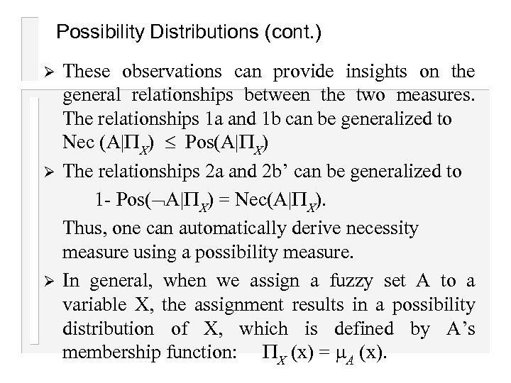 Possibility Distributions (cont. ) Ø Ø Ø These observations can provide insights on the general relationships between the two measures. The relationships 1 a and 1 b can be generalized to Nec (A| X) Pos(A| X) The relationships 2 a and 2 b’ can be generalized to 1 - Pos( A| X) = Nec(A| X). Thus, one can automatically derive necessity measure using a possibility measure. In general, when we assign a fuzzy set A to a variable X, the assignment results in a possibility distribution of X, which is defined by A’s membership function: X (x) = A (x).
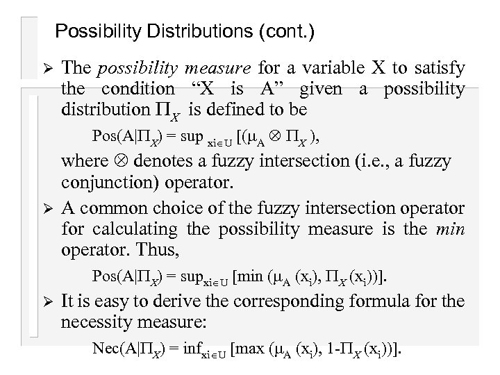 Possibility Distributions (cont. ) Ø The possibility measure for a variable X to satisfy the condition “X is A” given a possibility distribution X is defined to be Pos(A| X) = sup xi U [( A X ), Ø where denotes a fuzzy intersection (i. e. , a fuzzy conjunction) operator. A common choice of the fuzzy intersection operator for calculating the possibility measure is the min operator. Thus, Pos(A| X) = supxi U [min ( A (xi), X (xi))]. Ø It is easy to derive the corresponding formula for the necessity measure: Nec(A| X) = infxi U [max ( A (xi), 1 - X (xi))].
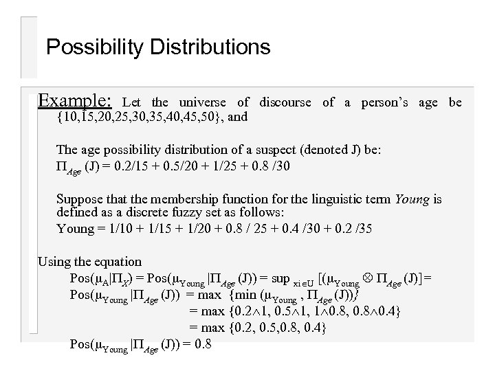 Possibility Distributions Example: Let the universe of discourse of a person’s age be {10, 15, 20, 25, 30, 35, 40, 45, 50}, and The age possibility distribution of a suspect (denoted J) be: Age (J) = 0. 2/15 + 0. 5/20 + 1/25 + 0. 8 /30 Suppose that the membership function for the linguistic term Young is defined as a discrete fuzzy set as follows: Young = 1/10 + 1/15 + 1/20 + 0. 8 / 25 + 0. 4 /30 + 0. 2 /35 Using the equation Pos( A| X) = Pos( Young | Age (J)) = sup xi U [( Young Age (J)]= Pos( Young | Age (J)) = max {min ( Young , Age (J))} = max {0. 2 1, 0. 5 1, 1 0. 8, 0. 8 0. 4} = max {0. 2, 0. 5, 0. 8, 0. 4} Pos( Young | Age (J)) = 0. 8
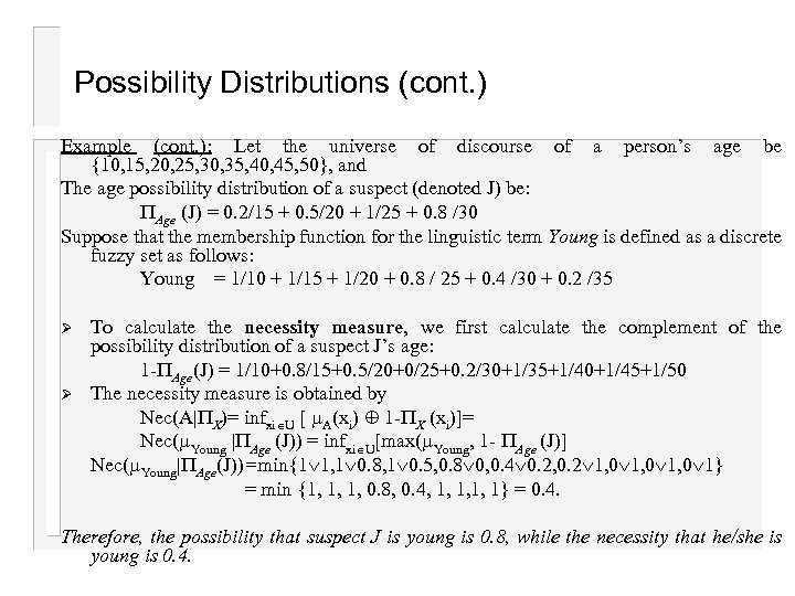 Possibility Distributions (cont. ) Example (cont. ): Let the universe of discourse of a person’s age be {10, 15, 20, 25, 30, 35, 40, 45, 50}, and The age possibility distribution of a suspect (denoted J) be: Age (J) = 0. 2/15 + 0. 5/20 + 1/25 + 0. 8 /30 Suppose that the membership function for the linguistic term Young is defined as a discrete fuzzy set as follows: Young = 1/10 + 1/15 + 1/20 + 0. 8 / 25 + 0. 4 /30 + 0. 2 /35 Ø Ø To calculate the necessity measure, we first calculate the complement of the possibility distribution of a suspect J’s age: 1 - Age(J) = 1/10+0. 8/15+0. 5/20+0/25+0. 2/30+1/35+1/40+1/45+1/50 The necessity measure is obtained by Nec(A| X)= infxi U [ A(xi) 1 - X (xi)]= Nec( Young | Age (J)) = infxi U[max( Young, 1 - Age (J)] Nec( Young| Age(J))=min{1 1, 1 0. 8, 1 0. 5, 0. 8 0, 0. 4 0. 2, 0. 2 1, 0 1} = min {1, 1, 1, 0. 8, 0. 4, 1, 1} = 0. 4. Therefore, the possibility that suspect J is young is 0. 8, while the necessity that he/she is young is 0. 4.
 Fuzzy If-Then Rules Ø Ø Ø There are two different kinds of fuzzy rules: Fuzzy mapping rules and Fuzzy implication rules. A fuzzy mapping rule describes an association; therefore, its fuzzy relation is constructed from the Cartesian product of its antecedent fuzzy condition and its consequent fuzzy condition. A fuzzy implication rule, however, describes a generalized logic implication; therefore, its fuzzy relation needs to be constructed from the semantics of a generalization to implication in multi-valued logic.
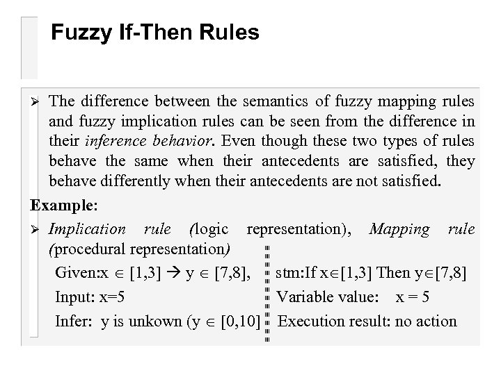 Fuzzy If-Then Rules The difference between the semantics of fuzzy mapping rules and fuzzy implication rules can be seen from the difference in their inference behavior. Even though these two types of rules behave the same when their antecedents are satisfied, they behave differently when their antecedents are not satisfied. Example: Ø Implication rule (logic representation), Mapping rule (procedural representation) Given: x [1, 3] y [7, 8], stm: If x [1, 3] Then y [7, 8] Input: x=5 Variable value: x = 5 Infer: y is unkown (y [0, 10] Execution result: no action Ø
 Fuzzy Mapping Rules Ø The needs to approximate a function of interest is often due to one or more of the following reasons: 1) The mathematical structure of the function is not precisely known. 2) The function is so complex that finding its precise mathematical form is either impossible or practically infeasible due to its high cost. 3) Even if finding the function is not impractical, implementing the function in its precise mathematical form in a product or service may be too costly. This is particularly important for low cost high volume products (e. g. , automobiles, cameras, and many other consumer products).
 Fuzzy Mapping Rules Ø Ø Fuzzy rule-based function approximation is a partition-based technique. The partition-based approximation techniques approximate a function by partitioning the input space of the function and approximate the function in each partitioned region separately (e. g. , piecewise linear approximation).
 Fuzzy Mapping Rules Ø Ø Ø Because each fuzzy rule approximates a small segment of the function, the entire function is approximated by a set of fuzzy mapping rules. We refer to such a collection of fuzzy mapping rules as fuzzy rule-based models or simply fuzzy models (describing a mapping (i. e. , function) from a set of input variables to a set of output variables. ) Example: a fuzzy model of the stock market can be used to predict future changes of the IMKB average. Ø A fuzzy control model of a petrochemical process can be used to predict the future state of the process.
 Fuzzy Mapping Rules Ø Ø Ø A fuzzy model can be defined as a model that is obtained by fusing multiple local models that are associated with fuzzy subspaces of the given input space. The result of fusing multiple local models is usually a fuzzy conclusion, which is converted to a crisp final output through a defuzzification process. The main difference between fuzzy and nonfuzzy rules for function approximation lies in their “interpolative reasoning” capability, which allows the output of multiple fuzzy rules to be fused for a given input.
 Fuzzy Mapping Rules Ø The four major concepts in fuzzy rule-based models thus are as follows: 1. Fuzzy partition, 2. Mapping of fuzzy subregion to local models, 3. Fusion of multiple local models, 4. Defuzzification.
 Fuzzy partition A fuzzy partition of a space is a collection of fuzzy subspaces whose boundaries partially overlap and whose union is the entire space. Ø Formally, a fuzzy partition of a space as a collection of fuzzy subspace Ai of S that satisfies the following condition: Ai(x) = 1, x S. Ø That is, for any element of the space, its membership degree in all subspaces always adds up to 1. Ø
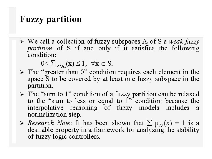 Fuzzy partition Ø Ø We call a collection of fuzzy subspaces Ai of S a weak fuzzy partition of S if and only if it satisfies the following condition: 0< Ai(x) 1, x S. The “greater than 0” condition requires each element in the space S to be covered by at least one fuzzy subspace in the partition. The “sum to 1” condition of a fuzzy partition can be relaxed to the “sum to less or equal to 1” condition because the interpolative reasoning of fuzzy models includes a normalization step. Research Note: It has been shown that Ai(x) = 1 is a desirable property in a framework for analyzing the stability of fuzzy logic controllers.
 Mapping a Fuzzy Subspace to a Local Model A local model for a subspace of the entire input space describes the system’s inputoutput mapping relationship in the small subspace. Ø In contrast, a global model for an input space describes the system’s input-output relationship for the entire input space. Ø Because the scope of the local model is smaller than that of a global model, it is usually easier to develop a local model. Ø
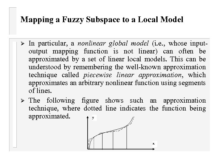 Mapping a Fuzzy Subspace to a Local Model Ø Ø In particular, a nonlinear global model (i. e. , whose inputoutput mapping function is not linear) can often be approximated by a set of linear local models. This can be understood by remembering the well-known approximation technique called piecewise linear approximation, which approximates an arbitrary nonlinear function using segments of lines. The following figure shows such an approximation technique, where dotted line indicates the function being approximated. y x
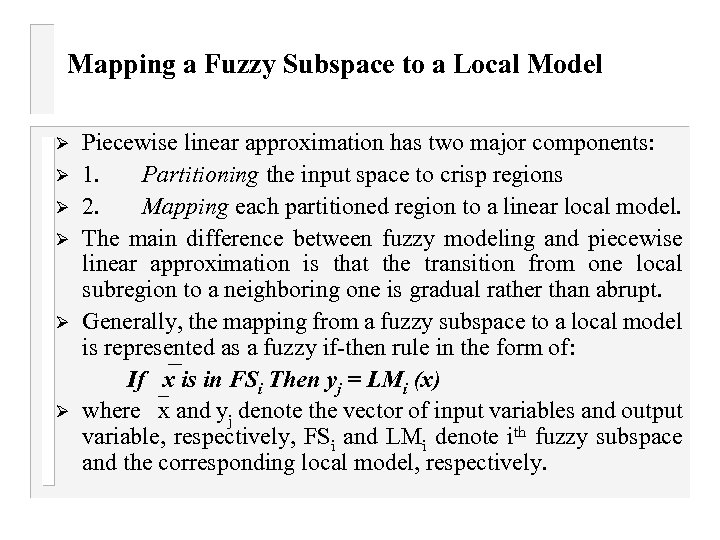 Mapping a Fuzzy Subspace to a Local Model Ø Ø Ø Piecewise linear approximation has two major components: 1. Partitioning the input space to crisp regions 2. Mapping each partitioned region to a linear local model. The main difference between fuzzy modeling and piecewise linear approximation is that the transition from one local subregion to a neighboring one is gradual rather than abrupt. Generally, the mapping from a fuzzy subspace to a local model is represented as a fuzzy if-then rule in the form of: If x is in FSi Then yj = LMi (x) where x and yj denote the vector of input variables and output variable, respectively, FSi and LMi denote ith fuzzy subspace and the corresponding local model, respectively.
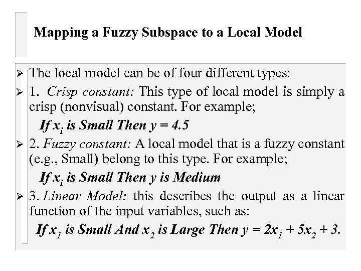 Mapping a Fuzzy Subspace to a Local Model Ø Ø The local model can be of four different types: 1. Crisp constant: This type of local model is simply a crisp (nonvisual) constant. For example; If xi is Small Then y = 4. 5 2. Fuzzy constant: A local model that is a fuzzy constant (e. g. , Small) belong to this type. For example; If xi is Small Then y is Medium 3. Linear Model: this describes the output as a linear function of the input variables, such as: If x 1 is Small And x 2 is Large Then y = 2 x 1 + 5 x 2 + 3.
 Fusion of local models through interpolative reasoning Ø Ø Fuzzy models use interpolative reasoning to fuse multiple local models into a global model. The basic idea behind interpolative reasoning is analogous to drawing a conclusion from a panel of experts, each of whom is specialized in a subarea of the entire problem. Each expert’s opinion is associated with a weight, which reflects the degree to which the current situation is in the expert’s specialized area. These weighted opinions are combined to form an overall opinion.
 Fusion of local models through interpolative reasoning In this analogy, an expert corresponds to a fuzzy if-then rule, the specialized subarea of the expert corresponds to the fuzzy subspace associated with the if-part of the rule. Ø The weight of an expert’s opinion is determined by the degree to which the current situation belongs to the subspace. Ø
 Defuzzification Ø Ø Ø We may interpret a possibility distribution either through linguistic approximation, or through defuzzification. The former gives a qualitative interpretation, while the latter gives a quantitative summary and is more commonly used in fuzzy logic applications, i. e. , industrial applications. Given a possibility distribution of a fuzzy model’s output, defuzzification amounts to selecting a single representative value that captures the essential meaning of the given distribution. There are three common defuzzification techniques: mean of maximum, center of area, and height.
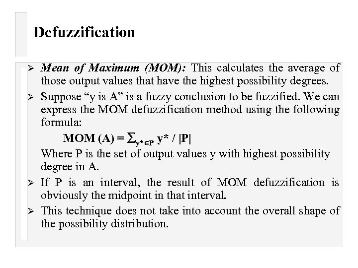 Defuzzification Ø Ø Mean of Maximum (MOM): This calculates the average of those output values that have the highest possibility degrees. Suppose “y is A” is a fuzzy conclusion to be fuzzified. We can express the MOM defuzzification method using the following formula: MOM (A) = y* P y* / |P| Where P is the set of output values y with highest possibility degree in A. If P is an interval, the result of MOM defuzzification is obviously the midpoint in that interval. This technique does not take into account the overall shape of the possibility distribution.
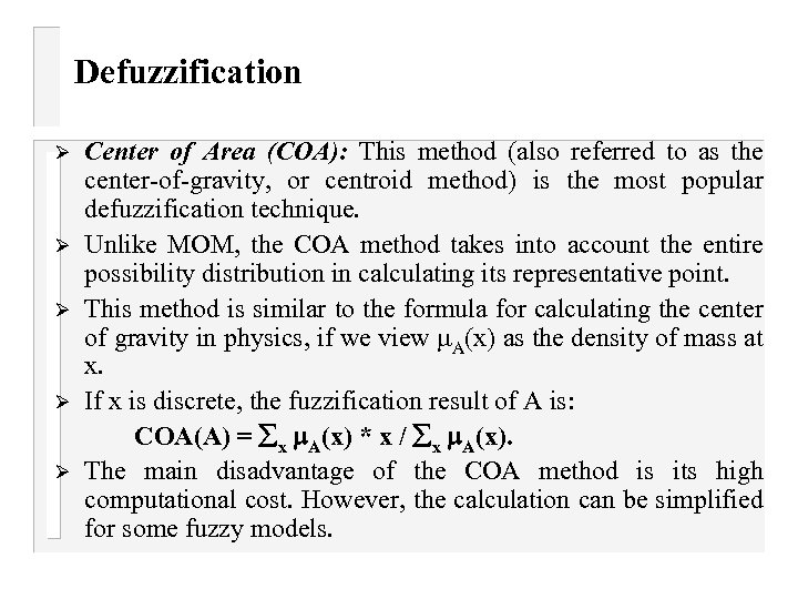 Defuzzification Ø Ø Ø Center of Area (COA): This method (also referred to as the center-of-gravity, or centroid method) is the most popular defuzzification technique. Unlike MOM, the COA method takes into account the entire possibility distribution in calculating its representative point. This method is similar to the formula for calculating the center of gravity in physics, if we view A(x) as the density of mass at x. If x is discrete, the fuzzification result of A is: COA(A) = x A(x) * x / x A(x). The main disadvantage of the COA method is its high computational cost. However, the calculation can be simplified for some fuzzy models.
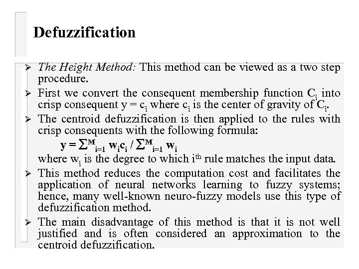 Defuzzification Ø Ø Ø The Height Method: This method can be viewed as a two step procedure. First we convert the consequent membership function Ci into crisp consequent y = ci where ci is the center of gravity of Ci. The centroid defuzzification is then applied to the rules with crisp consequents with the following formula: y = Mi=1 wici / Mi=1 wi where wi is the degree to which ith rule matches the input data. This method reduces the computation cost and facilitates the application of neural networks learning to fuzzy systems; hence, many well-known neuro-fuzzy models use this type of defuzzification method. The main disadvantage of this method is that it is not well justified and is often considered an approximation to the centroid defuzzification.
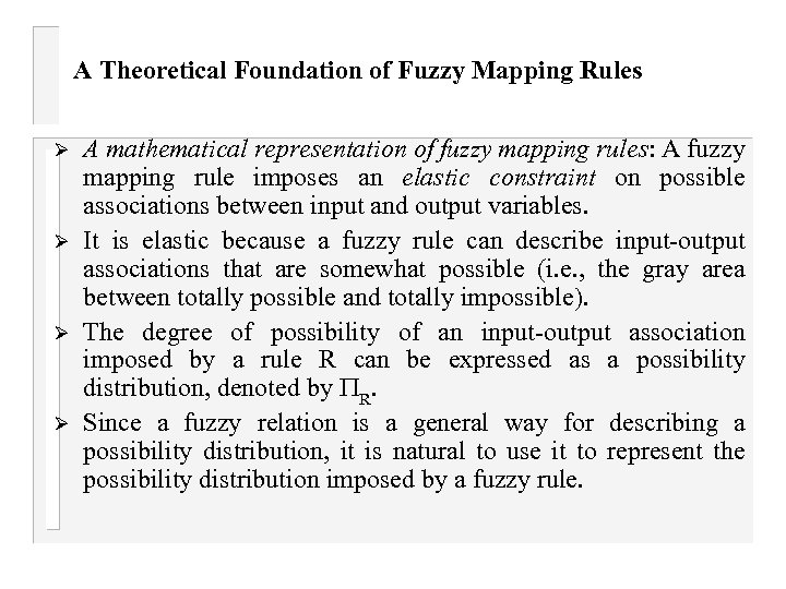 A Theoretical Foundation of Fuzzy Mapping Rules Ø Ø A mathematical representation of fuzzy mapping rules: A fuzzy mapping rule imposes an elastic constraint on possible associations between input and output variables. It is elastic because a fuzzy rule can describe input-output associations that are somewhat possible (i. e. , the gray area between totally possible and totally impossible). The degree of possibility of an input-output association imposed by a rule R can be expressed as a possibility distribution, denoted by R. Since a fuzzy relation is a general way for describing a possibility distribution, it is natural to use it to represent the possibility distribution imposed by a fuzzy rule.
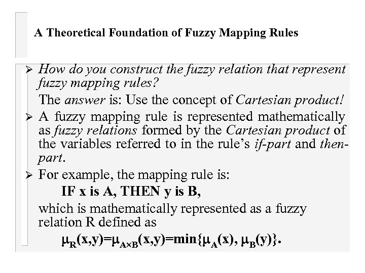 A Theoretical Foundation of Fuzzy Mapping Rules Ø Ø Ø How do you construct the fuzzy relation that represent fuzzy mapping rules? The answer is: Use the concept of Cartesian product! A fuzzy mapping rule is represented mathematically as fuzzy relations formed by the Cartesian product of the variables referred to in the rule’s if-part and thenpart. For example, the mapping rule is: IF x is A, THEN y is B, which is mathematically represented as a fuzzy relation R defined as R(x, y)= A B(x, y)=min{ A(x), B(y)}.
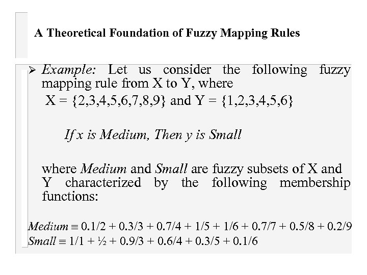 A Theoretical Foundation of Fuzzy Mapping Rules Ø Example: Let us consider the following fuzzy mapping rule from X to Y, where X = {2, 3, 4, 5, 6, 7, 8, 9} and Y = {1, 2, 3, 4, 5, 6} If x is Medium, Then y is Small where Medium and Small are fuzzy subsets of X and Y characterized by the following membership functions: Medium 0. 1/2 + 0. 3/3 + 0. 7/4 + 1/5 + 1/6 + 0. 7/7 + 0. 5/8 + 0. 2/9 Small 1/1 + ½ + 0. 9/3 + 0. 6/4 + 0. 3/5 + 0. 1/6
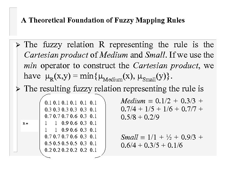 A Theoretical Foundation of Fuzzy Mapping Rules Ø Ø The fuzzy relation R representing the rule is the Cartesian product of Medium and Small. If we use the min operator to construct the Cartesian product, we have R(x, y) = min{ Medium(x), Small(y)}. The resulting fuzzy relation representing the rule is R 0. 1 0. 3 0. 1 0. 7 0. 6 0. 3 0. 1 1 1 0. 9 0. 6 0. 3 0. 1 0. 7 0. 6 0. 3 0. 1 0. 5 0. 3 0. 1 0. 2 0. 1 Medium 0. 1/2 + 0. 3/3 + 0. 7/4 + 1/5 + 1/6 + 0. 7/7 + 0. 5/8 + 0. 2/9 Small 1/1 + ½ + 0. 9/3 + 0. 6/4 + 0. 3/5 + 0. 1/6
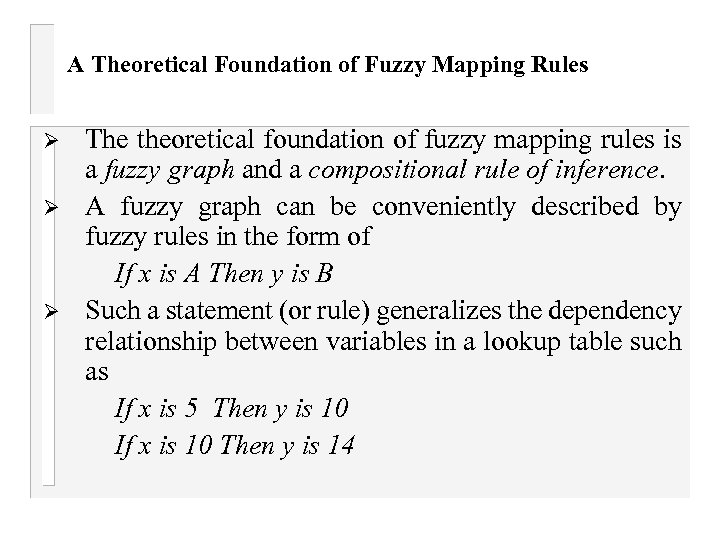 A Theoretical Foundation of Fuzzy Mapping Rules Ø Ø Ø The theoretical foundation of fuzzy mapping rules is a fuzzy graph and a compositional rule of inference. A fuzzy graph can be conveniently described by fuzzy rules in the form of If x is A Then y is B Such a statement (or rule) generalizes the dependency relationship between variables in a lookup table such as If x is 5 Then y is 10 If x is 10 Then y is 14
 A Theoretical Foundation of Fuzzy Mapping Rules Ø Ø 1. 2. A set of such dependencies form a functional mapping from x to y. Generalizing point-to-point mappings to a mapping from fuzzy sets to fuzzy sets introduces two benefits. We can reduce the total number of point-to-point rules required for approximating a function Using words in fuzzy rules makes it easier to capture, understand, and communicate the underlying human knowledge.
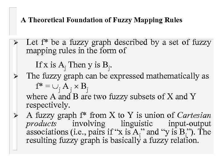 A Theoretical Foundation of Fuzzy Mapping Rules Ø Ø Ø Let f* be a fuzzy graph described by a set of fuzzy mapping rules in the form of If x is Aj Then y is Bj. The fuzzy graph can be expressed mathematically as f* = j A j Bj where A and B are two fuzzy subsets of X and Y respectively. A fuzzy graph f* from X to Y is union of Cartesian products involving linguistic input-output associations (i. e. , pairs if “x is Ai” and “y is Bi”). The resulting fuzzy graph is basically a fuzzy relation.
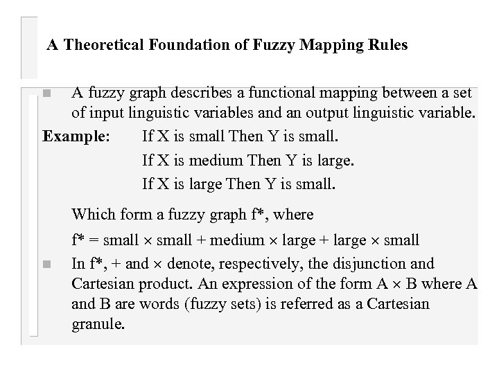 A Theoretical Foundation of Fuzzy Mapping Rules A fuzzy graph describes a functional mapping between a set of input linguistic variables and an output linguistic variable. Example: If X is small Then Y is small. If X is medium Then Y is large. If X is large Then Y is small. n Which form a fuzzy graph f*, where n f* = small + medium large + large small In f*, + and denote, respectively, the disjunction and Cartesian product. An expression of the form A B where A and B are words (fuzzy sets) is referred as a Cartesian granule.
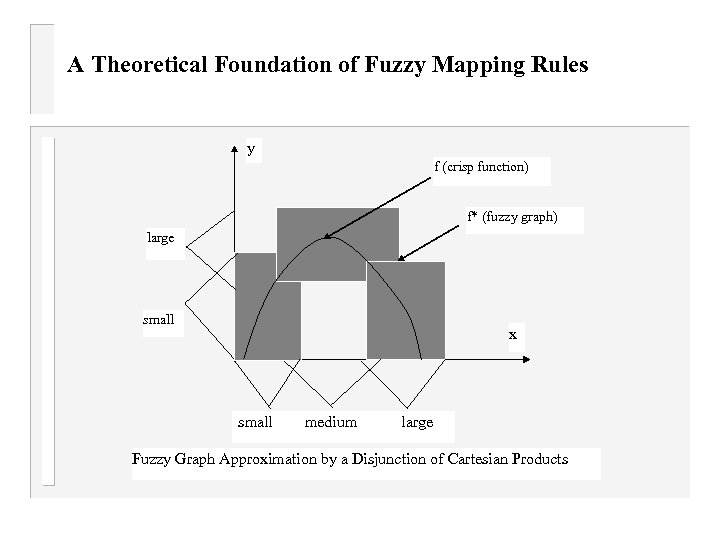 A Theoretical Foundation of Fuzzy Mapping Rules y f (crisp function) f* (fuzzy graph) large small x small medium large Fuzzy Graph Approximation by a Disjunction of Cartesian Products
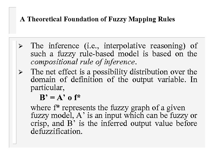 A Theoretical Foundation of Fuzzy Mapping Rules Ø Ø The inference (i. e. , interpolative reasoning) of such a fuzzy rule-based model is based on the compositional rule of inference. The net effect is a possibility distribution over the domain of definition of the output variable. In particular, B’ = A’ o f* where f* represents the fuzzy graph of a given fuzzy model, A’ is an input which can be fuzzy or crisp, and B’ is the inferred output value before defuzzification.
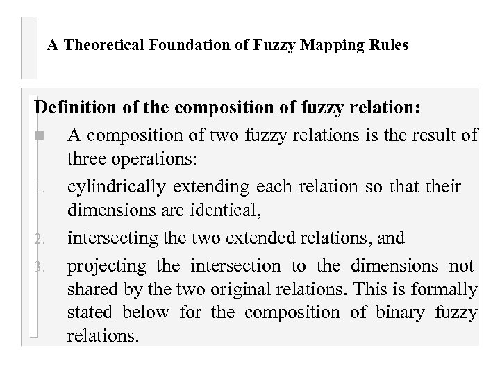 A Theoretical Foundation of Fuzzy Mapping Rules Definition of the composition of fuzzy relation: n A composition of two fuzzy relations is the result of three operations: 1. cylindrically extending each relation so that their dimensions are identical, 2. intersecting the two extended relations, and 3. projecting the intersection to the dimensions not shared by the two original relations. This is formally stated below for the composition of binary fuzzy relations.
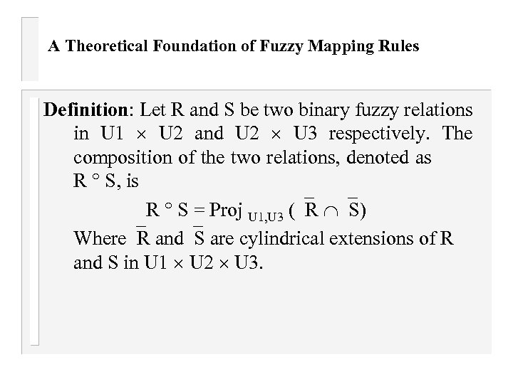 A Theoretical Foundation of Fuzzy Mapping Rules Definition: Let R and S be two binary fuzzy relations in U 1 U 2 and U 2 U 3 respectively. The composition of the two relations, denoted as R S, is R S = Proj U 1, U 3 ( R S) Where R and S are cylindrical extensions of R and S in U 1 U 2 U 3.
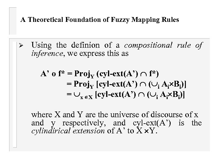 A Theoretical Foundation of Fuzzy Mapping Rules Ø Using the definion of a compositional rule of inference, we express this as A’ o f* = Proj. Y (cyl-ext(A’) f*) = Proj. Y [cyl-ext(A’) ( i Ai Bi)] = x X [cyl-ext(A’) ( i Ai Bi)] where X and Y are the universe of discourse of x and y respectively, and cyl-ext(A’) is the cylindirical extension of A’ to X Y.
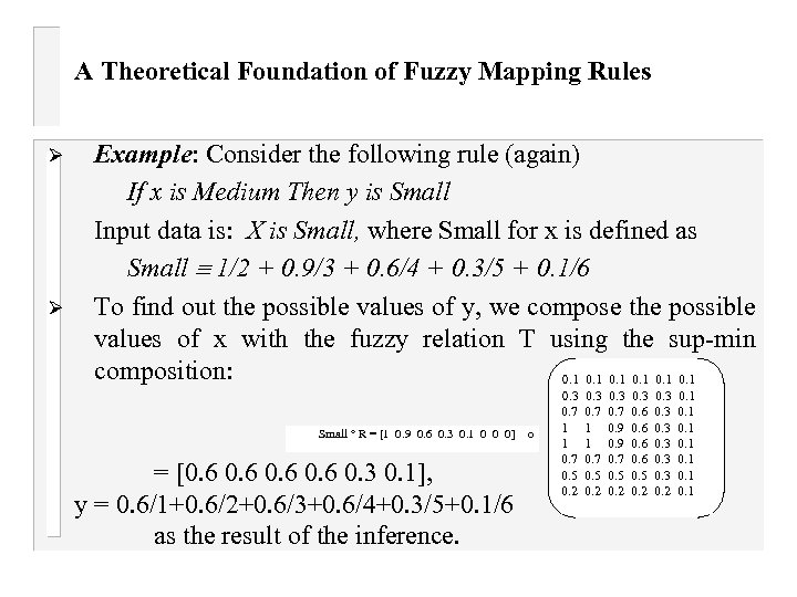 A Theoretical Foundation of Fuzzy Mapping Rules Ø Ø Example: Consider the following rule (again) If x is Medium Then y is Small Input data is: X is Small, where Small for x is defined as Small 1/2 + 0. 9/3 + 0. 6/4 + 0. 3/5 + 0. 1/6 To find out the possible values of y, we compose the possible values of x with the fuzzy relation T using the sup-min composition: 0. 1 0. 1 Small R = [1 0. 9 0. 6 0. 3 0. 1 0 0 0] o = [0. 6 0. 3 0. 1], y = 0. 6/1+0. 6/2+0. 6/3+0. 6/4+0. 3/5+0. 1/6 as the result of the inference. 0. 3 0. 1 0. 7 0. 6 0. 3 0. 1 1 1 0. 9 0. 6 0. 3 0. 1 0. 7 0. 6 0. 3 0. 1 0. 5 0. 3 0. 1 0. 2 0. 1
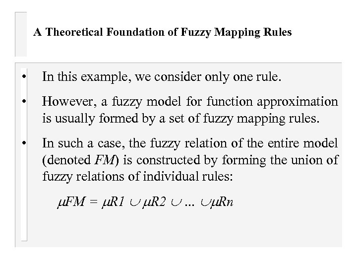 A Theoretical Foundation of Fuzzy Mapping Rules • In this example, we consider only one rule. • However, a fuzzy model for function approximation is usually formed by a set of fuzzy mapping rules. • In such a case, the fuzzy relation of the entire model (denoted FM) is constructed by forming the union of fuzzy relations of individual rules: FM = R 1 R 2 … Rn
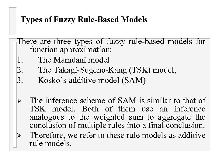 Types of Fuzzy Rule-Based Models There are three types of fuzzy rule-based models for function approximation: 1. The Mamdani model 2. The Takagi-Sugeno-Kang (TSK) model, 3. Kosko’s additive model (SAM) Ø Ø The inference scheme of SAM is similar to that of TSK model. Both of them use an inference analogous to the weighted sum to aggregate the conclusion of multiple rules into a final conclusion. Therefore, we refer to these rule models as additive rule models.
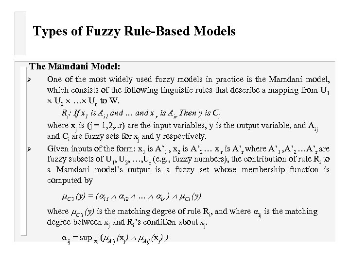 Types of Fuzzy Rule-Based Models The Mamdani Model: Ø Ø One of the most widely used fuzzy models in practice is the Mamdani model, which consists of the following linguistic rules that describe a mapping from U 1 U 2 … Ur to W. Ri: If x 1 is Ai 1 and … and x r is Air Then y is Ci where xj is (j = 1, 2, . . r) are the input variables, y is the output variable, and Aij and Ci are fuzzy sets for xj and y respectively. Given inputs of the form: x 1 is A’ 1 , x 2 is A’ 2 … x r is A’r where A’ 1 , A’ 2 …A’r are fuzzy subsets of U 1, U 2, …, Ur (e. g. , fuzzy numbers), the contribution of rule Ri to a Mamdani model’s output is a fuzzy set whose membership function is computed by C’i (y) = ( i 1 i 2 … ir ) Ci (y) where C’i (y) is the matching degree of rule Ri, and where ij is the matching degree between xj and Ri’s condition about xj. ij = sup xj ( A’j (xj) Aij (xj) )
 Types of Fuzzy Rule-Based Models and denotes the “min” operator. This is the “clipping inference method. Ø Ø Ø The final output of the model is the aggregation of outputs from all rules using the max operator. C (y) = max ( C’ 1(y), C’ 2(y), . . . , C’m(y)) Notice that the output C is a fuzzy set. This output can be defuzzified into a crisp output using one of the defuzzification techniques. The Mamdani model can be derived from the following operators: 1) Sup-min composition 2) Min for Cartesian product 3) Min for conjunctive conditions in rules 4) Max for aggregating multiple rules
 Types of Fuzzy Rule-Based Models Ø Ø Ø One of the main advantages of the TSK model is that it can approximate a function using fewer rules. In contrast, the Mamdani model combines inference results of rules using superimposition, not addition. Hence nonadditive rule model. The Mamdani and SAM use rules whose consequent part is a fuzzy set (uses a fuzzy constant as its rule’s local model). The TSK model uses a rule whose then part is a linear model (uses a linear local model). The fundamental difference between the Mamdani and SAM lies in the choice of composition, conjunction, and disjunction operators in their reasoning (inference mechanism).
 Fuzzy Implication Rules Ø Ø Ø Any logic system has two major components: 1. a formal language for constructing statements about the world, 2. a set of inference mechanisms for inferring additional statements about the world from those already given. Fuzzy logic is the most commonly used reasoning scheme in applications of fuzzy logic (narrow sense). The subject is complicated by the fact that there isn’t a unique definition of fuzzy implications.
 Fuzzy Implication Rules Ø Ø An important goal of fuzzy logic is to be able to make reasonable inference even when the condition of an implication rule is partially satisfied. This capability is sometimes referred to as approximate reasoning. This is achieved in fuzzy logic by two related techniques: 1. representing the meaning of a fuzzy implication rule using a fuzzy relation, and 2. obtaining an inferred conclusion by applying the compositional rule of inference to the fuzzy implication relation.
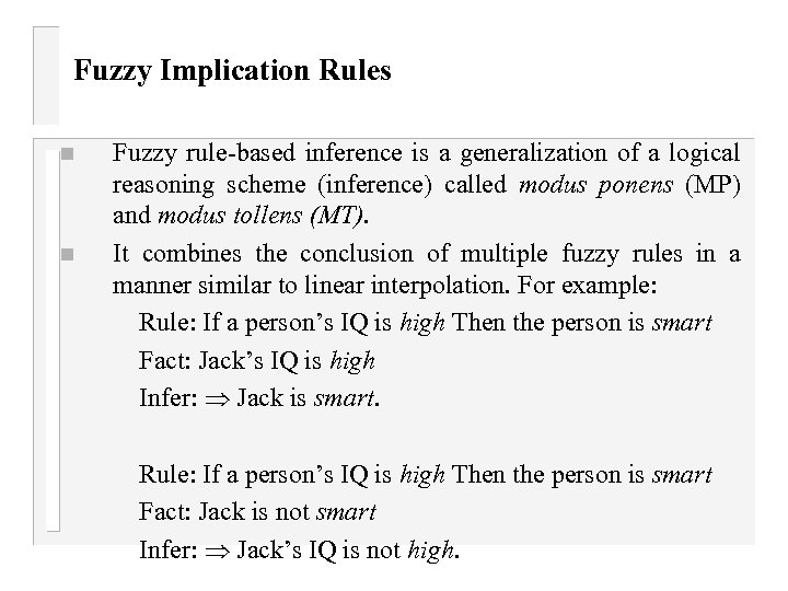 Fuzzy Implication Rules n n Fuzzy rule-based inference is a generalization of a logical reasoning scheme (inference) called modus ponens (MP) and modus tollens (MT). It combines the conclusion of multiple fuzzy rules in a manner similar to linear interpolation. For example: Rule: If a person’s IQ is high Then the person is smart Fact: Jack’s IQ is high Infer: Jack is smart. Rule: If a person’s IQ is high Then the person is smart Fact: Jack is not smart Infer: Jack’s IQ is not high.
 Fuzzy Implication Rules n n n First, these inferences insist on perfect matching. However, common sense reasoning suggest that we can infer “Jack is more or less smart” when the “Jack’s IQ is more or less high” is given. Secondly, these inferences cannot handle uncertainty. For instance, if Jack told us his IQ is high but cannot provide documents supporting the claim, we may be somewhat uncertain about the claim. Under such a circumstance, however, ordinary logic cannot reason about the uncertainty.
 Fuzzy Implication Rules n n These limitations motivated L. A. Zadeh to develop a reasoning scheme that generalizes classical logic so that It can conduct “common-sense” reasoning under partial matching, and It can reason about the certainty degree of a statement In particular, logic implications are generalized to allow partial matching. Rule: A person’s IQ is high the person is smart Fact: Jack’s IQ is somewhat high Infer: Jack is somewhat smart
 Fuzzy Implication Rules n n The second limitation of logic (i. e. , inability to deal with uncertainty) has motivated another extension to classical logic: multivalued logic. Since fuzzy logic also generalizes the truth-values in classical logic beyond true and false, it is related to multivalued logic. However, fuzzy logic differs from multivalued logic in that it also addresses the first limitation of logic (i. e. , restricted to perfect matching) by using linguistic variables in its antecedent. Consequently, the statement in the antecedent describes an elastic condition that can be partially satisfied.
 Fuzzy Implication Rules n 1. 2. 3. n Other approaches for reasoning under uncertainty include Bayesian probabilistic inference, Dempster-Shafer theory, nonmonotonic logic. Fuzzy logic, among these, is unique in that it addresses both the uncertainty management problem and the partial matching issue.
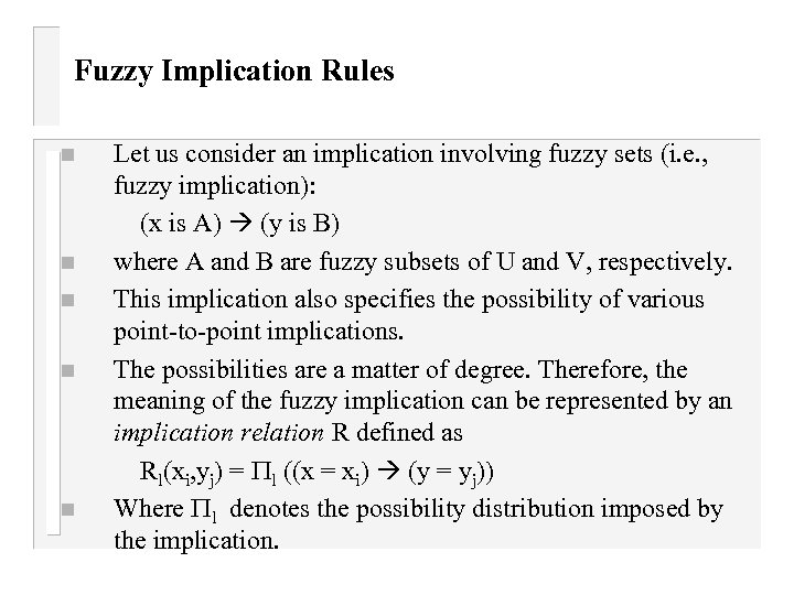 Fuzzy Implication Rules n n n Let us consider an implication involving fuzzy sets (i. e. , fuzzy implication): (x is A) (y is B) where A and B are fuzzy subsets of U and V, respectively. This implication also specifies the possibility of various point-to-point implications. The possibilities are a matter of degree. Therefore, the meaning of the fuzzy implication can be represented by an implication relation R defined as Rl(xi, yj) = l ((x = xi) (y = yj)) Where l denotes the possibility distribution imposed by the implication.
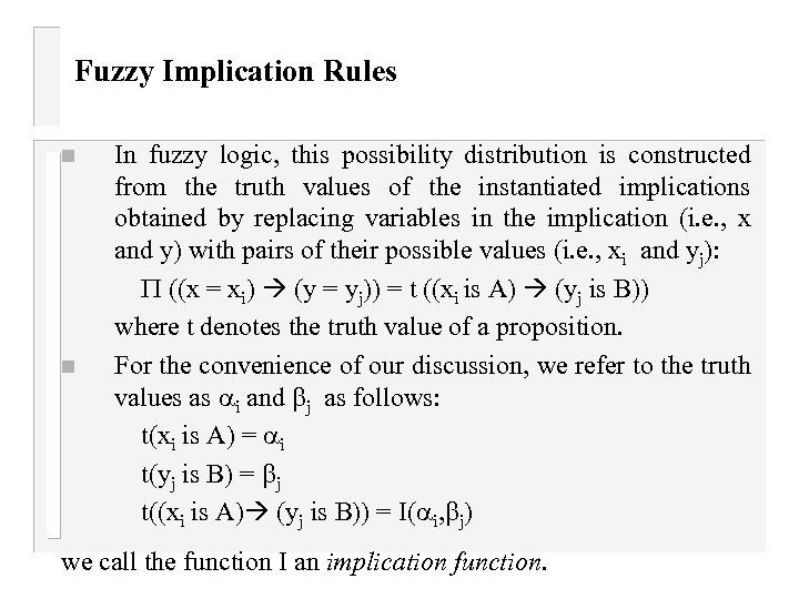 Fuzzy Implication Rules n n In fuzzy logic, this possibility distribution is constructed from the truth values of the instantiated implications obtained by replacing variables in the implication (i. e. , x and y) with pairs of their possible values (i. e. , xi and yj): ((x = xi) (y = yj)) = t ((xi is A) (yj is B)) where t denotes the truth value of a proposition. For the convenience of our discussion, we refer to the truth values as i and j as follows: t(xi is A) = i t(yj is B) = j t((xi is A) (yj is B)) = I( i, j) we call the function I an implication function.
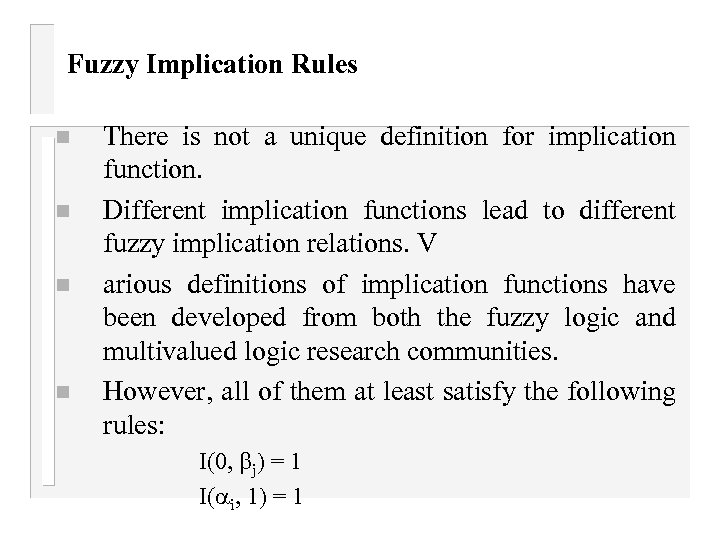 Fuzzy Implication Rules n n There is not a unique definition for implication function. Different implication functions lead to different fuzzy implication relations. V arious definitions of implication functions have been developed from both the fuzzy logic and multivalued logic research communities. However, all of them at least satisfy the following rules: I(0, j) = 1 I( i, 1) = 1
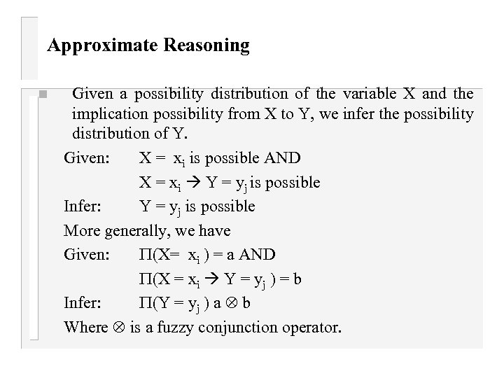 Approximate Reasoning n Given a possibility distribution of the variable X and the implication possibility from X to Y, we infer the possibility distribution of Y. Given: X = xi is possible AND X = xi Y = yj is possible Infer: Y = yj is possible More generally, we have Given: (X= xi ) = a AND (X = xi Y = yj ) = b Infer: (Y = yj ) a b Where is a fuzzy conjunction operator.
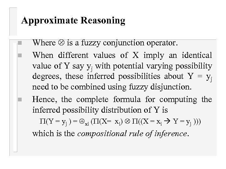 Approximate Reasoning n n n Where is a fuzzy conjunction operator. When different values of X imply an identical value of Y say yj with potential varying possibility degrees, these inferred possibilities about Y = yj need to be combined using fuzzy disjunction. Hence, the complete formula for computing the inferred possibility distribution of Y is (Y = yj ) = xi ( (X= xi) ((X = xi Y = yj ))) which is the compositional rule of inference.
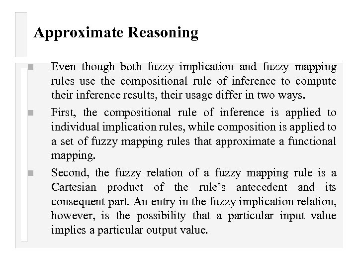 Approximate Reasoning n n n Even though both fuzzy implication and fuzzy mapping rules use the compositional rule of inference to compute their inference results, their usage differ in two ways. First, the compositional rule of inference is applied to individual implication rules, while composition is applied to a set of fuzzy mapping rules that approximate a functional mapping. Second, the fuzzy relation of a fuzzy mapping rule is a Cartesian product of the rule’s antecedent and its consequent part. An entry in the fuzzy implication relation, however, is the possibility that a particular input value implies a particular output value.
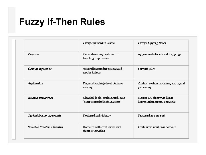 Fuzzy If-Then Rules Fuzzy Implication Rules Fuzzy Mapping Rules Purpose Generalizes implications for handling imprecision Approximate functional mappings Desired Inference Generalizes modus ponens and modus tollens Forward only Application Diagnostics, high-level decision making Control, system modeling, and signal processing Related Disciplines Classical logic, multivalued logic (other extended logic systems) System ID, piecewise linear interpolation, neural networks Typical Design Approach Designed individually Designed as a rule set Suitable Problem Domains with continuous and discrete variables Continuous nonlinear domains
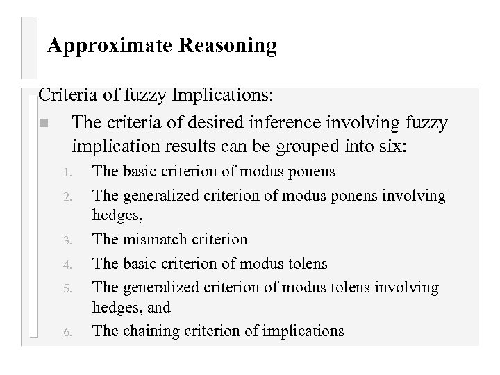 Approximate Reasoning Criteria of fuzzy Implications: n The criteria of desired inference involving fuzzy implication results can be grouped into six: 1. 2. 3. 4. 5. 6. The basic criterion of modus ponens The generalized criterion of modus ponens involving hedges, The mismatch criterion The basic criterion of modus tolens The generalized criterion of modus tolens involving hedges, and The chaining criterion of implications
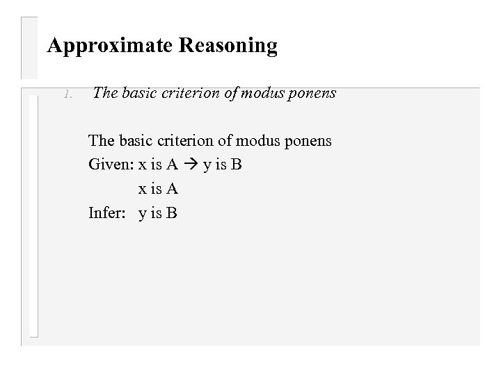 Approximate Reasoning 1. The basic criterion of modus ponens Given: x is A y is B x is A Infer: y is B
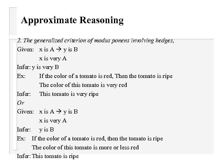 Approximate Reasoning 2. The generalized criterion of modus ponens involving hedges, Given: x is A y is B x is very A Infer: y is very B Ex: If the color of a tomato is red, Then the tomato is ripe The color of this tomato is very red Infer: This tomato is very ripe Or Given: x is A y is B x is very A Infer: y is B Ex: If the color of a tomato is red, then the tomato is ripe The color of this tomato is more or less red Infer: This tomato is ripe
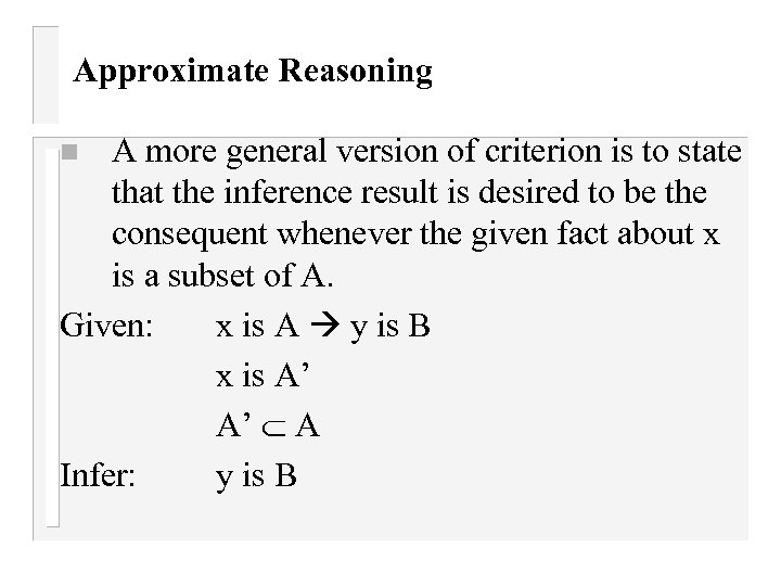 Approximate Reasoning A more general version of criterion is to state that the inference result is desired to be the consequent whenever the given fact about x is a subset of A. Given: x is A y is B x is A’ A’ A Infer: y is B n
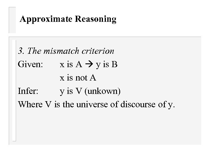 Approximate Reasoning 3. The mismatch criterion Given: x is A y is B x is not A Infer: y is V (unkown) Where V is the universe of discourse of y.
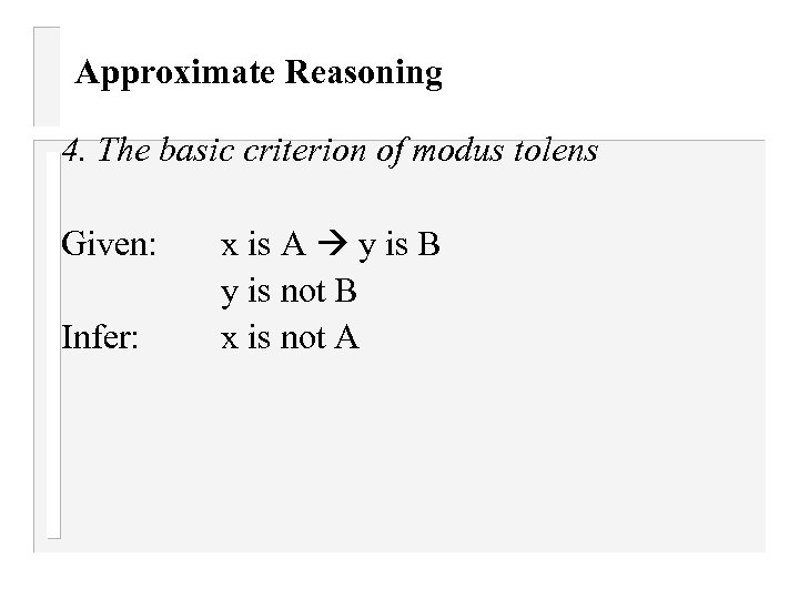 Approximate Reasoning 4. The basic criterion of modus tolens Given: Infer: x is A y is B y is not B x is not A
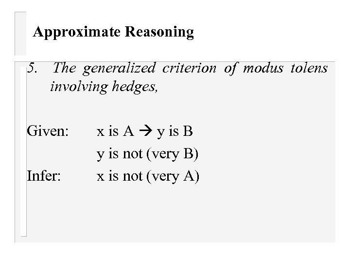 Approximate Reasoning 5. The generalized criterion of modus tolens involving hedges, Given: Infer: x is A y is B y is not (very B) x is not (very A)
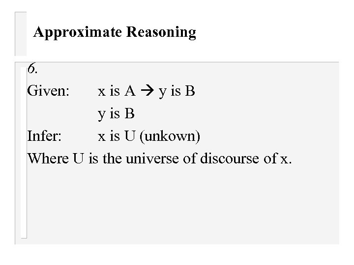 Approximate Reasoning 6. Given: x is A y is B Infer: x is U (unkown) Where U is the universe of discourse of x.
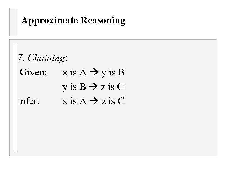 Approximate Reasoning 7. Chaining: Given: x is A y is B z is C Infer: x is A z is C
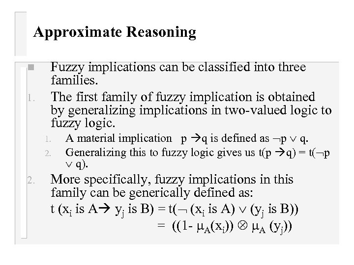 Approximate Reasoning n 1. Fuzzy implications can be classified into three families. The first family of fuzzy implication is obtained by generalizing implications in two-valued logic to fuzzy logic. 1. 2. A material implication p q is defined as p q. Generalizing this to fuzzy logic gives us t(p q) = t( p q). More specifically, fuzzy implications in this family can be generically defined as: t (xi is A yj is B) = t( (xi is A) (yj is B)) = ((1 - A(xi)) A (yj))
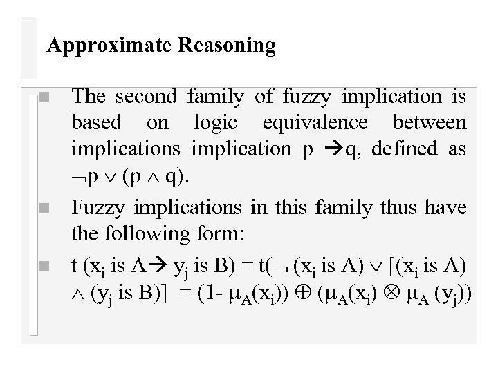 Approximate Reasoning n n n The second family of fuzzy implication is based on logic equivalence between implications implication p q, defined as p (p q). Fuzzy implications in this family thus have the following form: t (xi is A yj is B) = t( (xi is A) [(xi is A) (yj is B)] = (1 - A(xi)) ( A(xi) A (yj))
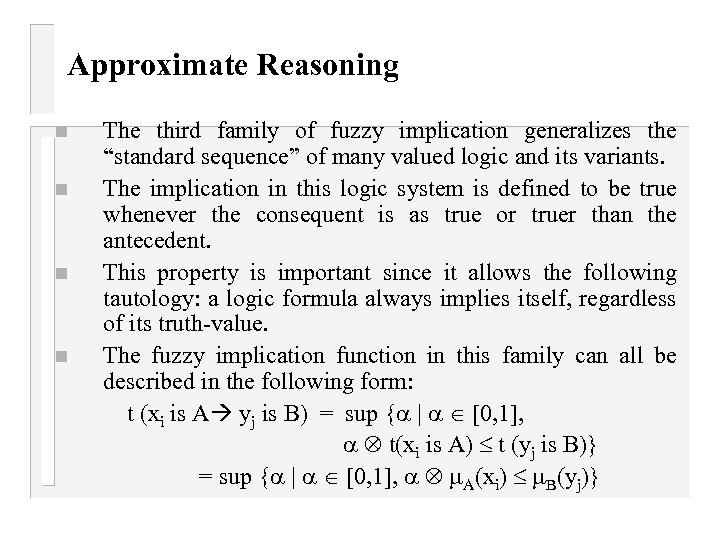 Approximate Reasoning n n The third family of fuzzy implication generalizes the “standard sequence” of many valued logic and its variants. The implication in this logic system is defined to be true whenever the consequent is as true or truer than the antecedent. This property is important since it allows the following tautology: a logic formula always implies itself, regardless of its truth-value. The fuzzy implication function in this family can all be described in the following form: t (xi is A yj is B) = sup { | [0, 1], t(xi is A) t (yj is B)} = sup { | [0, 1], A(xi) B(yj)}
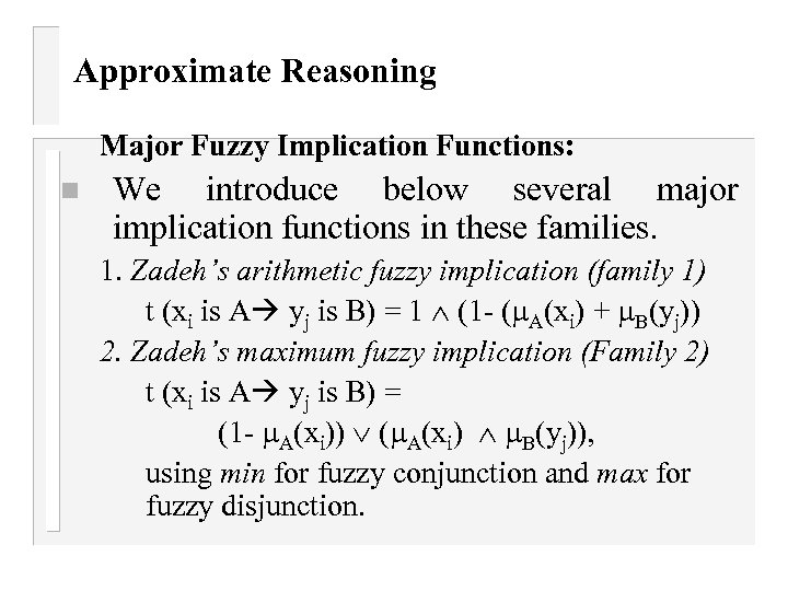 Approximate Reasoning Major Fuzzy Implication Functions: n We introduce below several major implication functions in these families. 1. Zadeh’s arithmetic fuzzy implication (family 1) t (xi is A yj is B) = 1 (1 - ( A(xi) + B(yj)) 2. Zadeh’s maximum fuzzy implication (Family 2) t (xi is A yj is B) = (1 - A(xi)) ( A(xi) B(yj)), using min for fuzzy conjunction and max for fuzzy disjunction.
 Approximate Reasoning
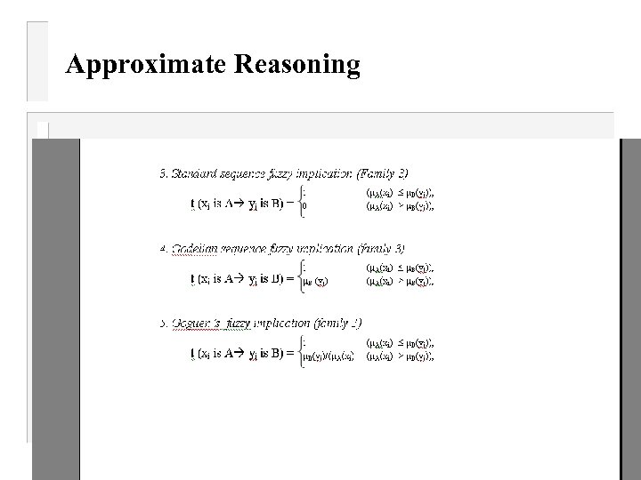
 Approximate Reasoning n n n All the latter three fuzzy implications came from multivalued logic systems. Even though implication functions in multivalued logic systems can be used for constructing fuzzy implication relations, approximate reasoning in fuzzy logic is fundamentally different from logic inference in multi-valued logic. Approximate reasoning infers possible values of a variable, whereas multivalued logic infers the truth-values of propositions. Approximate reasoning benefits from the following important concepts and techniques in fuzzy logic: the compositional rule of inference, fuzzy relations, and possibility distributions. Without them, approximate reasoning would not have been possible. Among the five fuzzy implication functions, the standard sequence fuzzy implication satisfies most criteria.


