11dd3b28d5cd3ec824da8d39fa814e81.ppt
- Количество слайдов: 36
 Introduction to Financial Economics Lecture Notes 12 Ch 1, 2 - Lengwiler 1
 Overview of the Course Introduction- Finance and its roots in economics- general equilibrium theory, microeconomics and macroeconomics. Contingent Claim Economies - commodity spaces, preferences, general equilibrium, representative agents. Asset Economies- financial assets, Radner economies, Arrow-Debreu pricing, complete and incomplete markets. Risky Decisions- expected utility paradigm. Static Finance Economy- risk sharing, representative v. NM agent, sdf’s, equilibrium price of risk and time. Dynamic Finance Economies- dynamic trading etc. Taking Theory to the Data: empirical papers. 2
 Some Background • Introduction to the foundations of modern finance theory linking it to roots in GE and economic theory. • Math Background: basics of vector spaces, statistics, maximization subject to constraints and calculus (Simon and Blume, 1994, Mathematics for Economists, WW Norton) is the level required. • Other Finance texts: Leroy and Werner, Danthine and Donaldson, Campbell, Lo and Mackinlay, Gollier, and Cochrane. • Classic texts: Huang and Litzenberger and Ingersoll. 3
 What is Financial Economics about? • Finance – How prices are determined in financial markets ? and How risk and capital is allocated across agents and across the economy ? • Individual agents take decisions about savings and investments with regard to the risk they can bear. • If markets work well, risk and capital will be allocated to projects that get the best risk return profile. • Finance theory also useful for policy analysis to assess welfare gains and losses. • Origins of Finance – draws on General Equilibrium Theory, Macroeconomics and Microeconomic theory. 4
 What is General Equilibrium about? • Describes the behavior of an economy - focusing at the optimal behavior of each member of the set of agents in the economy and looks for a point of mutual compatibility. • Underlying assumptions: – Agents do not interact with each other directly but through markets. – Markets are anonymous- only prices (or “exchange rates” for different commodities are posted) – Agents are small relative to the market i. e. there is perfect competition. • Such models are called Walrasian in honour of Leon Walras who was the first to formulate such a model. . 5
 Modern General Equilibrium theory • Modern GE theory-follows Arrow and Debreu- allows for a large number of goods and diverse preferences of individuals. • Establishes the conditions that guarantee the existence of an equilibrium. • Develops the properties of equilibrium allocations- or the famous Welfare Theorems. • Welfare Theorems- show that market equilibrium allocations and socially efficient allocations are, under some conditions, equivalent. • Radner etc. built financial markets into these modelsmaking possible the study of incomplete markets- book by Magill and Quinzi has all the details. 6
 Macroeconomic Origins • Keynesian macro-models do not feature individual agents or dynamics explicitly- focus on interaction between different aggregate variables- lack the individual optimization perspective. • Hicks’s version of Keynes’s model also lacks this perspective- has problems with endogenous determination of expectations. • Led to the rational expectations revolution in economicsto construct dynamic models of aggregate economic fluctuations based on individual decisions about shocks (mainly to technology). • Also led to the models with one agent and one good to get easily computable equilibria (Real Business Cycle literature). 7
 Origins of Finance • Finance started as a field of business administration. • Markowitz (1952) – offered a simple decision rule for investing in financial assets (m-v optimization). • Sharpe and others - Emphasis on the determinants of asset prices- showed that only that part of the risk is priced in equilibrium that covaries with the market (e. g. the CAPM). • Two main areas of asset pricing: Relative pricing i. e. pricing one asset relative to the price of another asset v. Absolute pricing which relates asset prices to fundamental or state variables in the economy. • Relative pricing- pricing of derivative securities-futures contracts priced relative to the underlying asset-many uses including in the commercial world. • Absolute pricing -What are the macroeconomic sources of risk in the economy that affect asset prices? Multifactor models like APT, Merton’s ICAPM etc. 8
 Finance • • • Traditional GE theory- describes properties of equilibrium allocations + existence and efficiency of equilibria. Macroeconomics- on the time series or dynamical properties of aggregate measures of economic activity. GE theory that focuses on explaining the prices of financial assets is equilibrium asset pricing theory. Stiglitz (1970, Re. Stud) connects finance closely with economic theory-leads later to Lucas (1987) tree model and Breeden CCAPM. First Welfare Theorem- use it to justify using a simple one-good and one-agent economy- adding v. NM utility theory we can allow for preferences etc. Finance economy- How changes in stochastic properties of endowments affect equilibrium prices of securities. 9
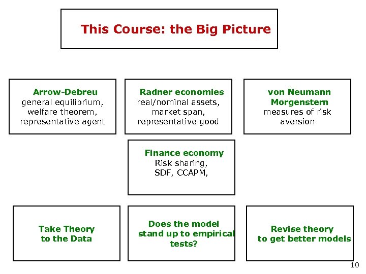 This Course: the Big Picture Arrow-Debreu general equilibrium, welfare theorem, representative agent Radner economies real/nominal assets, market span, representative good von Neumann Morgenstern measures of risk aversion Finance economy Risk sharing, SDF, CCAPM, Take Theory to the Data Does the model stand up to empirical tests? Revise theory to get better models 10
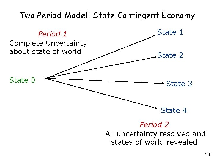
 Contingent Claim Economy • What is a commodity ? Defined by physical characteristics, geographical place of availability, time of availability. Example: an umbrella in London in the summer. • Fourth property- Conditionality-A good may or may not be useful conditional on a random (exogenous) event. • Example: An umbrella when it rains v. umbrella when it does not rain – are two different commodities. • Commodity- physical specification, place of availability, event contingent (in multi-period setting) or state contingent (two-period setting). 11
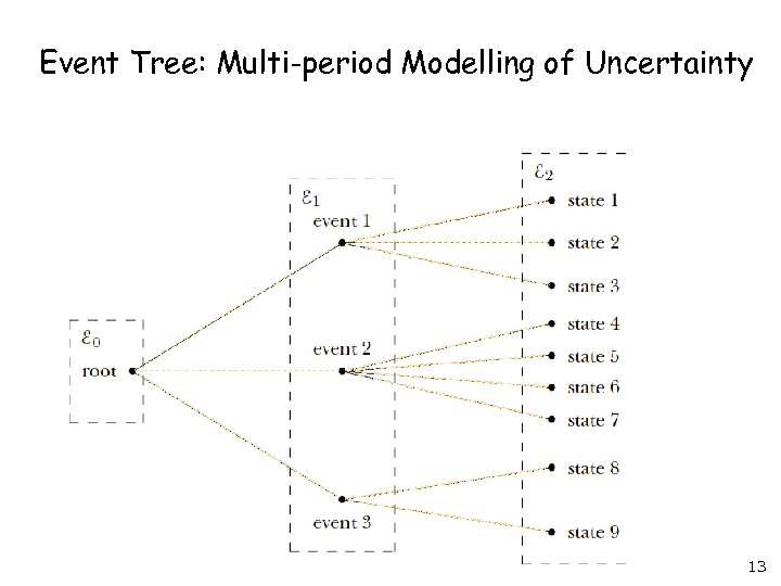
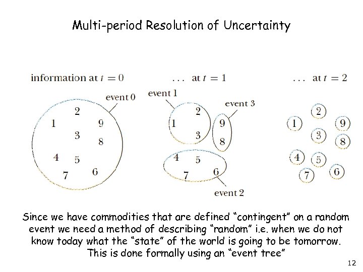 Multi-period Resolution of Uncertainty Since we have commodities that are defined “contingent” on a random event we need a method of describing “random” i. e. when we do not know today what the “state” of the world is going to be tomorrow. This is done formally using an “event tree” 12
 Event Tree: Multi-period Modelling of Uncertainty 13
 Two Period Model: State Contingent Economy Period 1 Complete Uncertainty about state of world State 0 State 1 State 2 State 3 State 4 Period 2 All uncertainty resolved and states of world revealed 14
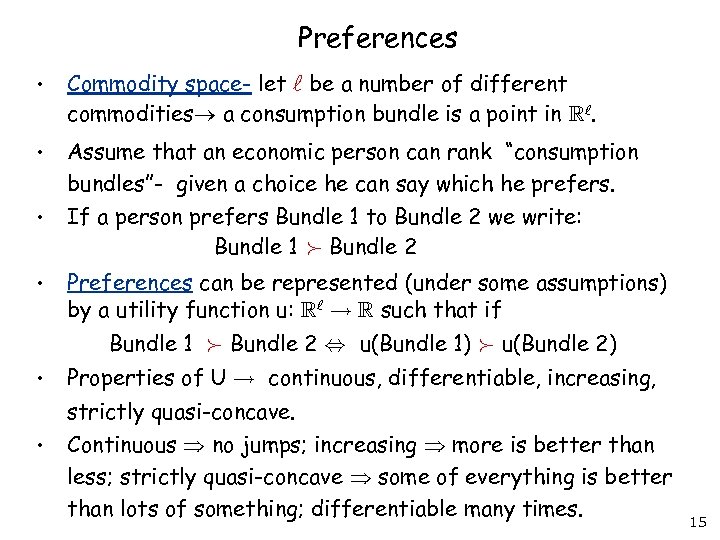 Preferences • Commodity space- let be a number of different commodities a consumption bundle is a point in . • Assume that an economic person can rank “consumption bundles”- given a choice he can say which he prefers. • If a person prefers Bundle 1 to Bundle 2 we write: Bundle 1 Bundle 2 • Preferences can be represented (under some assumptions) by a utility function u: such that if Bundle 1 Bundle 2 u(Bundle 1) u(Bundle 2) • • Properties of U continuous, differentiable, increasing, strictly quasi-concave. Continuous no jumps; increasing more is better than less; strictly quasi-concave some of everything is better than lots of something; differentiable many times. 15
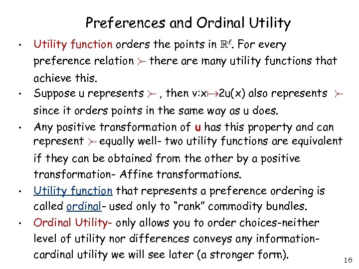 Preferences and Ordinal Utility • Utility function orders the points in . For every preference relation there are many utility functions that • achieve this. Suppose u represents , then v: x 2 u(x) also represents since it orders points in the same way as u does. • • • Any positive transformation of u has this property and can represent equally well- two utility functions are equivalent if they can be obtained from the other by a positive transformation- Affine transformations. Utility function that represents a preference ordering is called ordinal- used only to “rank” commodity bundles. Ordinal Utility- only allows you to order choices-neither level of utility nor differences conveys any informationcardinal utility we will see later (a stronger form). 16
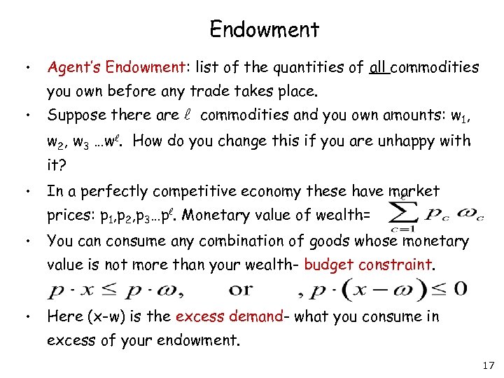 Endowment • Agent’s Endowment: list of the quantities of all commodities you own before any trade takes place. • Suppose there are commodities and you own amounts: w 1, w 2, w 3 …w. How do you change this if you are unhappy with it? • In a perfectly competitive economy these have market prices: p 1, p 2, p 3…p. Monetary value of wealth= • You can consume any combination of goods whose monetary value is not more than your wealth- budget constraint. • Here (x-w) is the excess demand- what you consume in excess of your endowment. 17
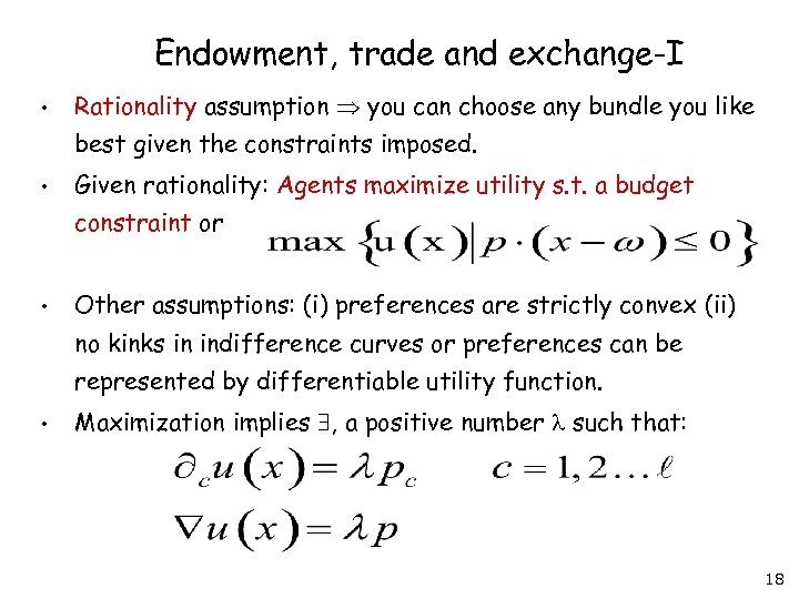 Endowment, trade and exchange-I • Rationality assumption you can choose any bundle you like best given the constraints imposed. • Given rationality: Agents maximize utility s. t. a budget constraint or • Other assumptions: (i) preferences are strictly convex (ii) no kinks in indifference curves or preferences can be represented by differentiable utility function. • Maximization implies , a positive number such that: 18
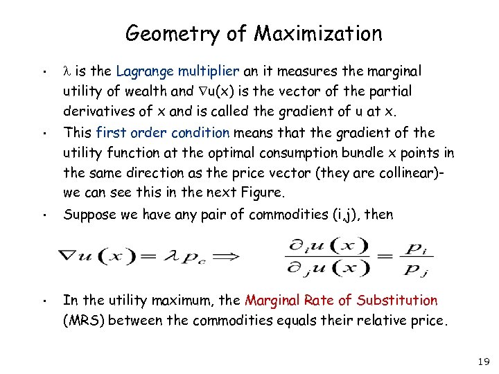 Geometry of Maximization • is the Lagrange multiplier an it measures the marginal utility of wealth and u(x) is the vector of the partial derivatives of x and is called the gradient of u at x. • This first order condition means that the gradient of the utility function at the optimal consumption bundle x points in the same direction as the price vector (they are collinear)we can see this in the next Figure. • Suppose we have any pair of commodities (i, j), then • In the utility maximum, the Marginal Rate of Substitution (MRS) between the commodities equals their relative price. 19
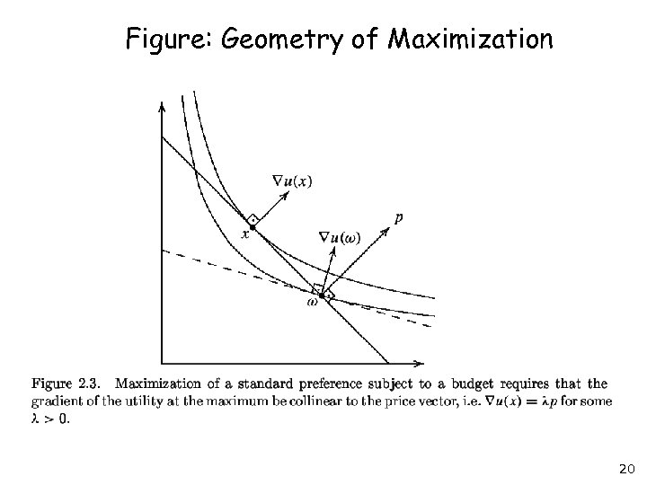 Figure: Geometry of Maximization 20
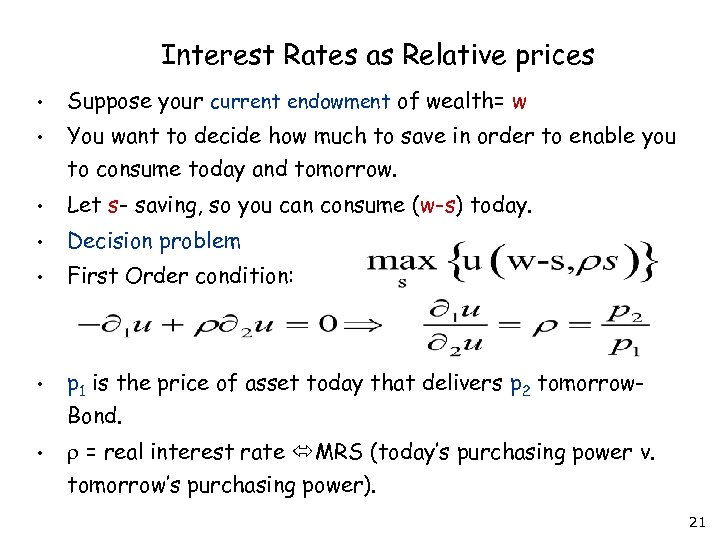 Interest Rates as Relative prices • Suppose your current endowment of wealth= w • You want to decide how much to save in order to enable you to consume today and tomorrow. • Let s- saving, so you can consume (w-s) today. • Decision problem • First Order condition: • p 1 is the price of asset today that delivers p 2 tomorrow. Bond. • = real interest rate MRS (today’s purchasing power v. tomorrow’s purchasing power). 21
 General Equilibrium • GE theory –concerns interaction of optimizing agents through markets. • Questions: Does and equilibrium exist? Is it unique? Are the equilibrium allocations efficient? • Finance (or macrofinance- asset pricing for example) not concerned with existence or equilibrium allocation. • Finance focuses on equilibrium prices and how they relate to utilities (average tastes) and (average) endowments. • What does “average” tastes mean? Aggregation Problem. • In GE theory – the R. A behaves the same everywhere-both at and off the “equilibrium”. • Finance - need agent who is- “local representative agent” or behaves like only at equilibrium- We now see how we can construct this local representative. 22
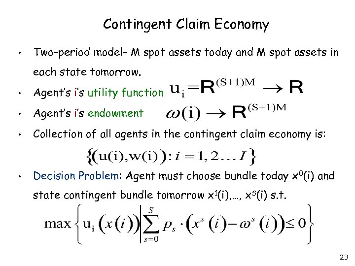 Contingent Claim Economy • Two-period model- M spot assets today and M spot assets in each state tomorrow. • Agent’s i’s utility function • Agent’s i’s endowment • Collection of all agents in the contingent claim economy is: • Decision Problem: Agent must choose bundle today x 0(i) and state contingent bundle tomorrow x 1(i), …, x. S(i) s. t. 23
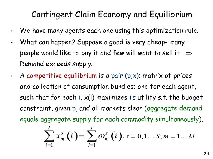 Contingent Claim Economy and Equilibrium • We have many agents each one using this optimization rule. • What can happen? Suppose a good is very cheap- many people would like to buy it and few will want to sell it Demand exceeds supply. • A competitive equilibrium is a pair (p, x); matrix of prices and collection of consumption bundles; one for each agent, such that for each i, x(i) maximizes i’s utility s. t. the budget constraint, given p, and all markets clear (aggregate demand equals aggregate supply for each commodity simultaneously). 24
 Some General Points • Step #1: How to construct a representative agent. • Step #2: How to go from many commodities into one aggregate commodity namely wealth. Objective: one-good and one-agent economy. • We want to use this to determine the macroeconomic determinants of asset prices. • Existence of equilibrium is an important issue in GE theorybut not in finance -we will not go into this in this course. • However here’s why this is important: A model should at least guarantee an an equilibrium-otherwise it is incomplete. • GE theory uses things like fixed point theorems to prove these things. ( see any text like Mas-Collel etc for details). 25
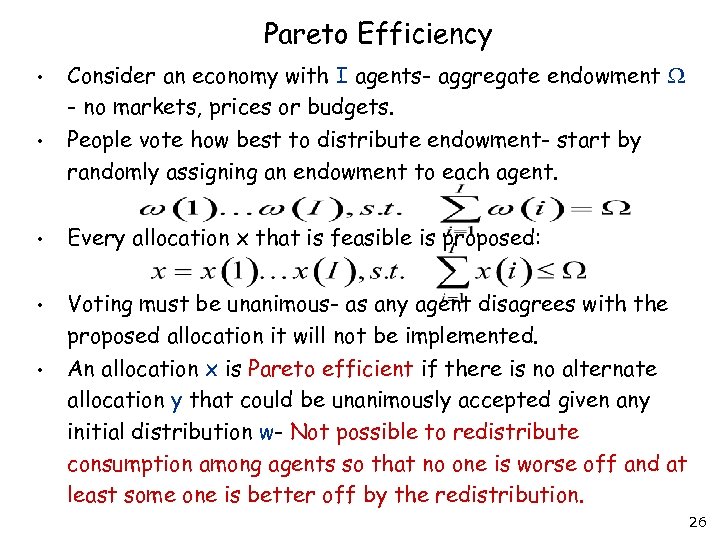 Pareto Efficiency • • Consider an economy with I agents- aggregate endowment - no markets, prices or budgets. People vote how best to distribute endowment- start by randomly assigning an endowment to each agent. • Every allocation x that is feasible is proposed: • Voting must be unanimous- as any agent disagrees with the proposed allocation it will not be implemented. An allocation x is Pareto efficient if there is no alternate allocation y that could be unanimously accepted given any initial distribution w- Not possible to redistribute consumption among agents so that no one is worse off and at least some one is better off by the redistribution. • 26
 First Welfare Theorem • Everyone is marginally identical in equilibrium- hence there are no further gains from trade and the equilibrium allocation is Pareto efficient. • Equilibrium allocations are Pareto efficient. Why? Everyone’s maximum indifference curve is tangent to the budget hyperplane in equilibrium no unexploited gains by trade. In other words, given a competitive equilibrium allocation there is no redistribution that would be accepted unanimously. So if we have: the utility functions of the agents + an aggregate endowment: We can the generate all Pareto efficient allocations with the help of a Social Welfare Function. A SWF is a weighted sum of individual utilities maximized subject to feasibility constraints. • • • 27
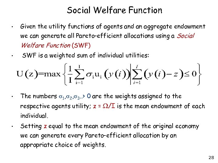 Social Welfare Function • Given the utility functions of agents and an aggregate endowment we can generate all Pareto-efficient allocations using a Social Welfare Function (SWF) • • SWF is a weighted sum of individual utilities: The numbers 1, 2, 3. . > 0 are the weights assigned to the respective agents utility; z = /I is the mean endowment of each individual. • Setting z equal to the mean endowment of the original economy we can generate every Pareto-efficient allocation by an appropriate choice of weights. 28
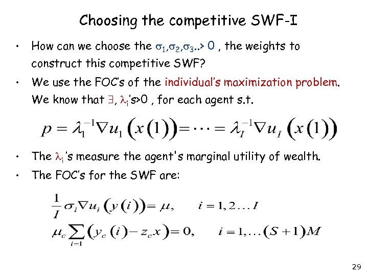 Choosing the competitive SWF-I • How can we choose the 1, 2, 3. . > 0 , the weights to construct this competitive SWF? • We use the FOC’s of the individual’s maximization problem. We know that , i’s>0 , for each agent s. t. • The i ’s measure the agent's marginal utility of wealth. • The FOC’s for the SWF are: 29
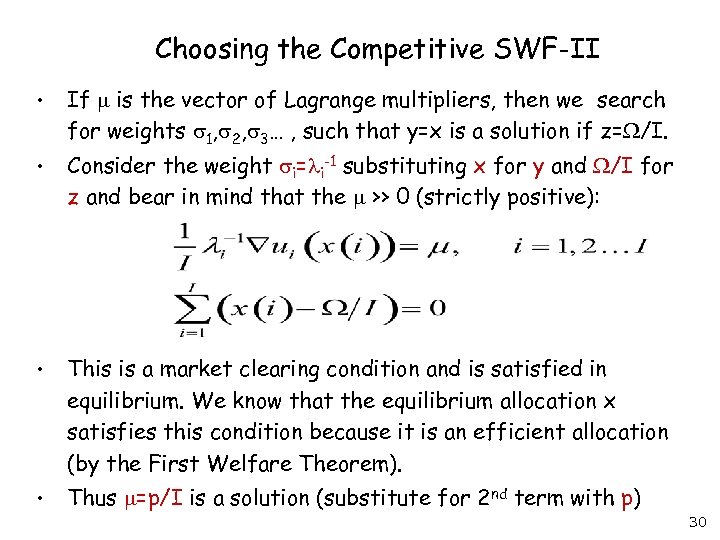 Choosing the Competitive SWF-II • If is the vector of Lagrange multipliers, then we search for weights 1, 2, 3… , such that y=x is a solution if z= /I. • Consider the weight i= i-1 substituting x for y and /I for z and bear in mind that the >> 0 (strictly positive): • This is a market clearing condition and is satisfied in equilibrium. We know that the equilibrium allocation x satisfies this condition because it is an efficient allocation (by the First Welfare Theorem). • Thus =p/I is a solution (substitute for 2 nd term with p) 30
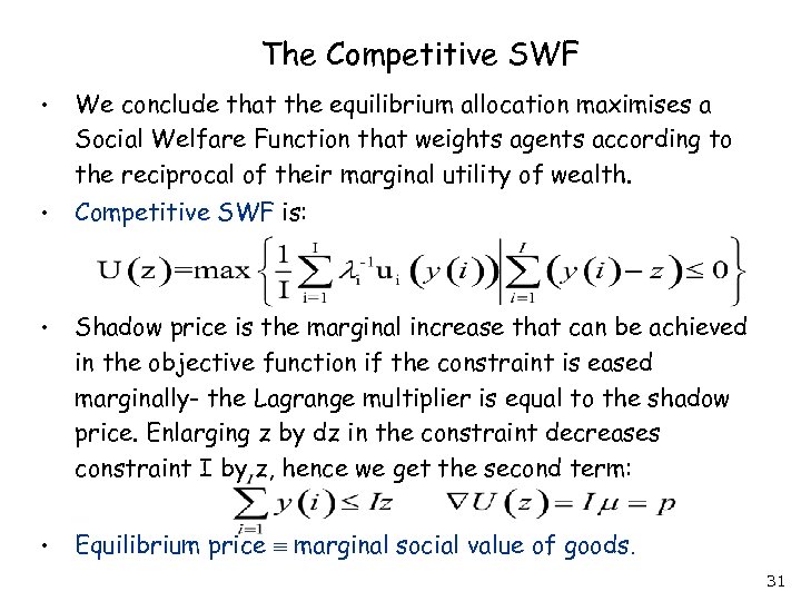 The Competitive SWF • We conclude that the equilibrium allocation maximises a Social Welfare Function that weights agents according to the reciprocal of their marginal utility of wealth. • Competitive SWF is: • Shadow price is the marginal increase that can be achieved in the objective function if the constraint is eased marginally- the Lagrange multiplier is equal to the shadow price. Enlarging z by dz in the constraint decreases constraint I by z, hence we get the second term: • Equilibrium price marginal social value of goods. 31
 Some Summing up • We studied an abstract contingent claim economy. • We defined a Pareto efficient allocation and a competitive equilibrium in a contingent claim economy. • A SWF is the value of a problem that maximizes a weighted sum of individual utilities subject to the material limitations of the economy. • An allocation is Pareto efficient if and only if it is the solution to some SWF. • A competitive equilibrium is a price-allocation pair in which all markets clear and ever agent maximizes utility subject to a budget constraint. • Key result: First Welfare Theorem- A competitive equilibrium allocation is Pareto efficient. 32
 Features of Representative Agents • • • Economist are interested in aggregate data that we can observe and societies utility function-not necessarily in an individuals endowment and decisions. If we have an economy (u, w) with I agents – to solve for a competitive equilibrium (p, x) would be cumbersome- we need to do this for every agent. If there is only one agent- we know the equilibrium allocation because there is nobody else to trade with- equilibrium prices are just the gradient of this agent’s utility function at his endowment point. Given a multi-agent economy (u, w) and a competitive equilibrium (p, x) we define a locally representative agent as an artificial agent (u 0, w 0) such that (p, x 0) is a competitive equilibrium of this oneagent economy (u 0, w 0). The equilibrium allocation is w 0 or it is no-trade situation in this one-agent economy. 33
 Representative Agents- some discussion • • • If we work with a representative agent we lose all information on the inter-personal equilibrium distribution- we don’t know who consumes what-however in finance we are not interested in this micro-information. An arbitrary representative agent: Take any utility function v and a point x where the FOC is achieved: v(x)= p, then letting =1, (v, x) is a representative agent. Why? Faced with prices p he will not wish to trade forming a oneperson general equilibrium. However this arbitrary R. A. is not very useful- he has no relation to the original data of the multi=person economy. How can we construct a representative from the data of the original economy? Use result of the Pareto efficiency of an equilibrium- everyone is marginally identical in equilibrium everyone is a representative agent in equilibrium. 34
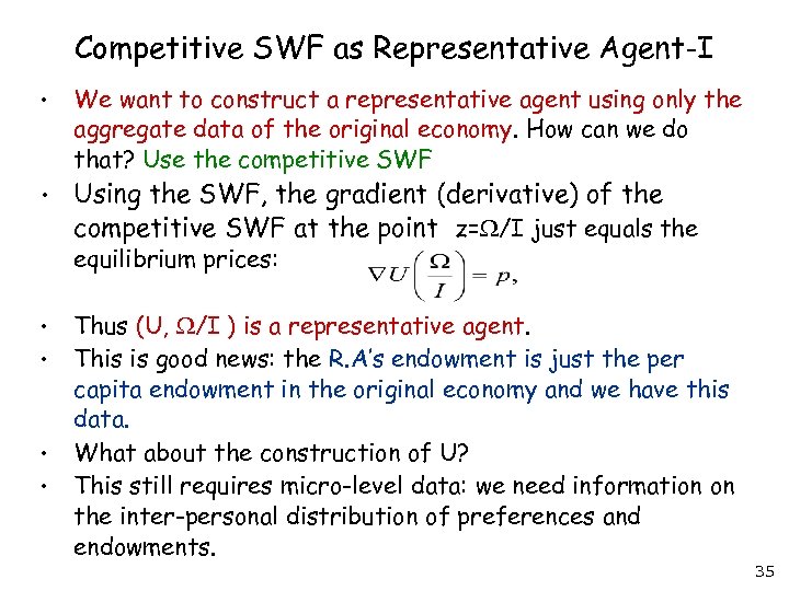 Competitive SWF as Representative Agent-I • • We want to construct a representative agent using only the aggregate data of the original economy. How can we do that? Use the competitive SWF Using the SWF, the gradient (derivative) of the competitive SWF at the point z= /I just equals the equilibrium prices: • • Thus (U, /I ) is a representative agent. This is good news: the R. A’s endowment is just the per capita endowment in the original economy and we have this data. What about the construction of U? This still requires micro-level data: we need information on the inter-personal distribution of preferences and endowments. 35
 Competitive SWF as Representative Agent-II • What about the construction of U? • We can estimate U or • We can assume that everyone has the same utility function u but different endowments w(i) and then use data on endowment distributions to compute U. • However we do not need to do this. • We next investigate a class of utility functions that can be aggregated without the knowledge of the distribution of endowments. • These arise from the von Neumann-Morgenstern utility theory- we look at this topic next. 36


