Introduction to Economics 1 Demand 2 Supply

Introduction to Economics

1. Demand 2. Supply 3. Market equilibrium 3/16/2018 2

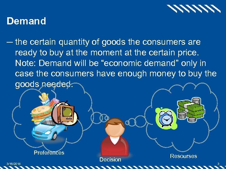Demand ─ the certain quantity of goods the consumers are ready to buy at the moment at the certain price. Note: Demand will be “economic demand” only in case the consumers have enough money to buy the goods needed. Preferences 3/16/2018 Decision Resourses 3

Law of downward-sloping demand: 2 reasons for it ─ When the price of commodity raises (ceteris paribus) buyers tend to buy less of the commodity. ─ Substitution effect: consumer substitutes the more expensive good by less expensive and therefore decreases his demand for it. ─ Income effect: when all the prices go up the consumer feels himself relatively poorer than before (i. e. real income goes down). In this respect he decreases his consumption. 3/16/2018 4

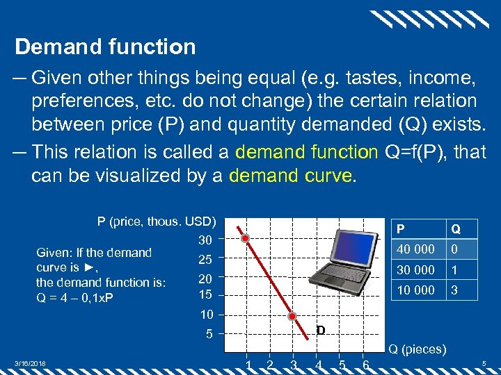Demand function ─ Given other things being equal (e. g. tastes, income, preferences, etc. do not change) the certain relation between price (P) and quantity demanded (Q) exists. ─ This relation is called a demand function Q=f(P), that can be visualized by a demand curve. P (price, thous. USD) 30 Given: If the demand 25 curve is ►, 20 the demand function is: 15 Q = 4 – 0, 1 x. P 10 P Q 40 000 0 30 000 1 10 000 3 D 5 Q (pieces) 3/16/2018 1 2 3 4 5 6 5

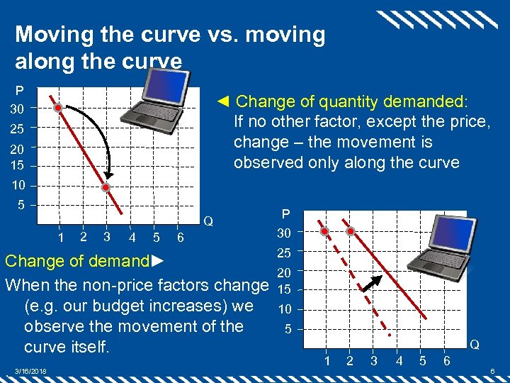Moving the curve vs. moving along the curve P 30 ◄ Change of quantity demanded: If no other factor, except the price, change – the movement is observed only along the curve 25 20 15 10 5 Q 1 2 3 4 5 6 Change of demand► When the non-price factors change (e. g. our budget increases) we observe the movement of the curve itself. . 3/16/2018 P 30 25 20 15 10 5 Q 1 2 3 4 5 6 6

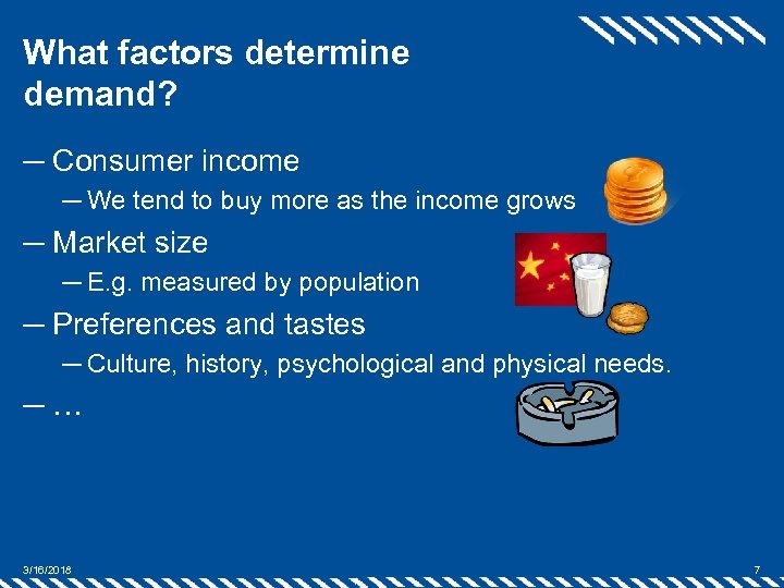What factors determine demand? ─ Consumer income ─ We tend to buy more as the income grows ─ Market size ─ E. g. measured by population ─ Preferences and tastes ─ Culture, history, psychological and physical needs. ─… 3/16/2018 7

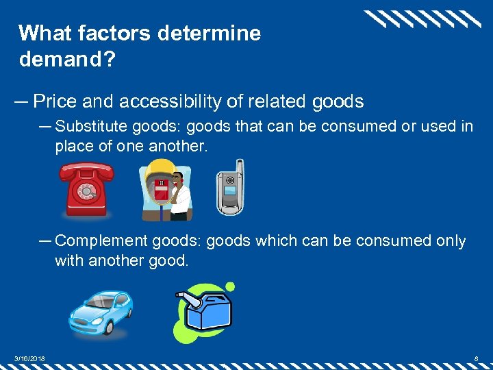What factors determine demand? ─ Price and accessibility of related goods ─ Substitute goods: goods that can be consumed or used in place of one another. ─ Complement goods: goods which can be consumed only with another good. 3/16/2018 8

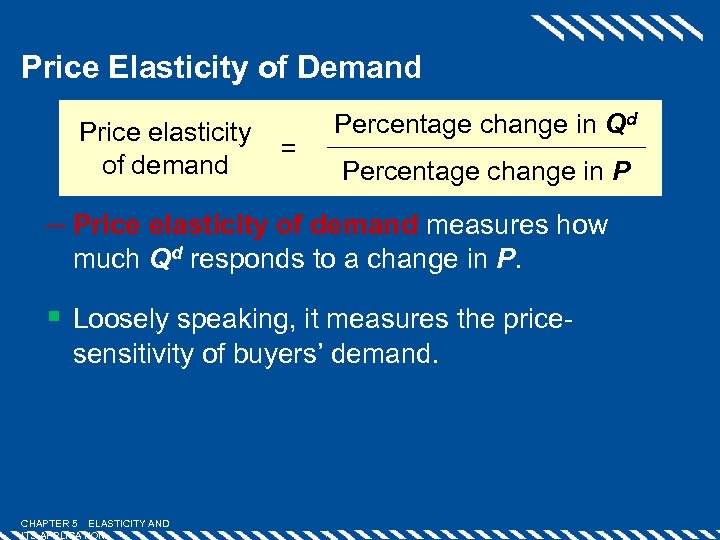Price Elasticity of Demand Price elasticity of demand = Percentage change in Qd Percentage change in P ─ Price elasticity of demand measures how much Qd responds to a change in P. § Loosely speaking, it measures the pricesensitivity of buyers’ demand. CHAPTER 5 ELASTICITY AND ITS APPLICATION

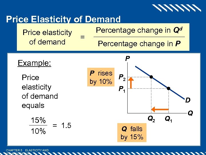Price Elasticity of Demand Price elasticity of demand Example: Price elasticity of demand equals 15% = 1. 5 10% CHAPTER 5 ELASTICITY AND ITS APPLICATION = Percentage change in Qd Percentage change in P P P rises P 2 by 10% P 1 D Q 2 Q falls by 15% Q 1 Q

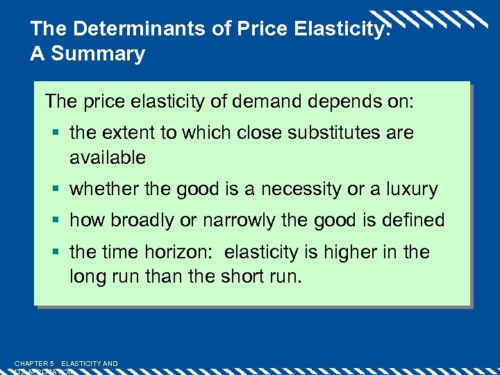The Determinants of Price Elasticity: A Summary The price elasticity of demand depends on: § the extent to which close substitutes are available § whether the good is a necessity or a luxury § how broadly or narrowly the good is defined § the time horizon: elasticity is higher in the long run than the short run. CHAPTER 5 ELASTICITY AND ITS APPLICATION

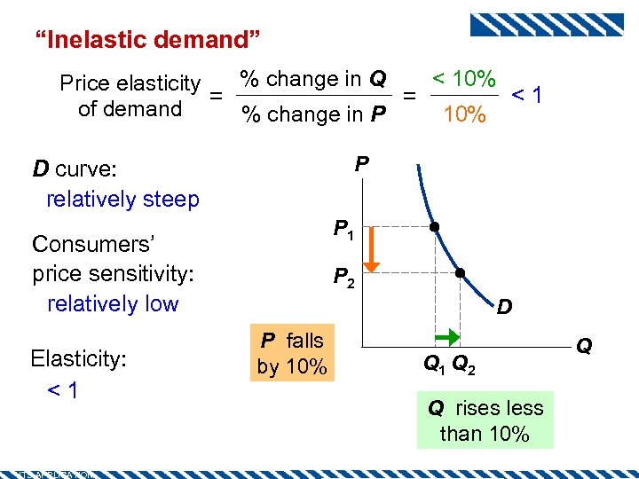“Inelastic demand” < 10% % change in Q Price elasticity <1 = = of demand 10% % change in P P D curve: relatively steep P 1 Consumers’ price sensitivity: relatively low Elasticity: <1 CHAPTER 5 ELASTICITY AND ITS APPLICATION P 2 D P falls by 10% Q 1 Q 2 Q rises less than 10% Q

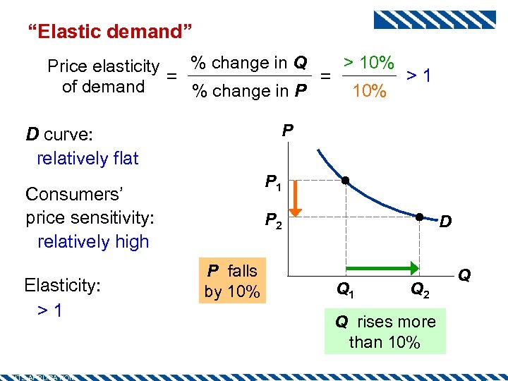“Elastic demand” > 10% % change in Q Price elasticity >1 = = of demand 10% % change in P P D curve: relatively flat P 1 Consumers’ price sensitivity: relatively high Elasticity: >1 CHAPTER 5 ELASTICITY AND ITS APPLICATION P 2 P falls by 10% D Q 1 Q 2 Q rises more than 10% Q

“Perfectly inelastic demand” (one extreme case) % change in Q Price elasticity = = of demand % change in P P D curve: vertical CHAPTER 5 ELASTICITY AND ITS APPLICATION 10% =0 D P 1 Consumers’ price sensitivity: 0 Elasticity: 0 0% P 2 P falls by 10% Q 1 Q changes by 0% Q

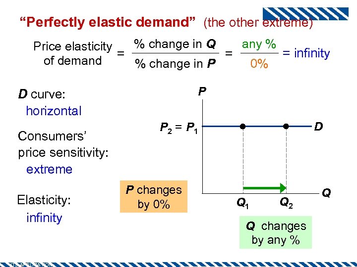“Perfectly elastic demand” (the other extreme) any % % change in Q Price elasticity = infinity = = of demand 0% % change in P P D curve: horizontal Consumers’ price sensitivity: extreme Elasticity: infinity CHAPTER 5 ELASTICITY AND ITS APPLICATION D P 2 = P 1 P changes by 0% Q 1 Q 2 Q changes by any % Q

What do we need price elasticity indicator for? ─ Company price policy before all: ─ Price discrimination: e. g. flight companies determine customer groups with different price elastic ties ─ Sales in the supermarkets 3/16/2018 16

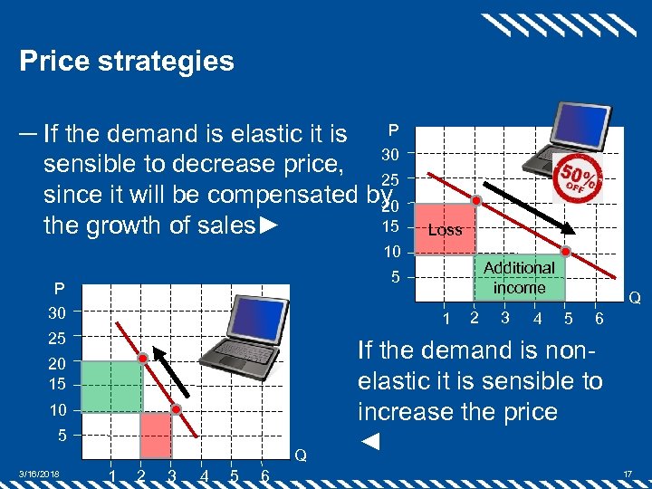Price strategies P ─ If the demand is elastic it is sensible to decrease price, 30 25 since it will be compensated by 20 15 the growth of sales► Loss 10 P 30 1 25 20 15 10 5 Q 3/16/2018 Additional income 5 1 2 3 4 5 6 2 3 4 Q 5 6 If the demand is nonelastic it is sensible to increase the price ◄ 17

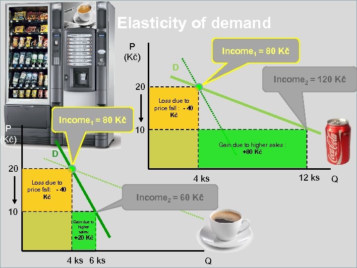Elasticity of demand P (Kč) Income 1 = 80 Kč D Income 2 = 120 Kč 20 Income 1 = 80 Kč P (Kč) Loss due to price fall : - 40 Kč 10 Gain due to higher sales : +80 Kč D 20 4 ks Loss due to price fall: - 40 Kč Income 2 = 60 Kč 10 Gain due to higher sales: +20 Kč 4 ks 6 ks Q 12 ks Q

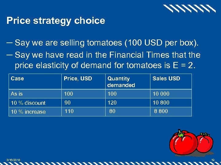Price strategy choice ─ Say we are selling tomatoes (100 USD per box). ─ Say we have read in the Financial Times that the price elasticity of demand for tomatoes is E = 2. Case Price, USD Quantity demanded Sales USD As is 100 10 000 10 % discount 90 120 10 800 10 % increase 110 80 8 800 3/16/2018 19

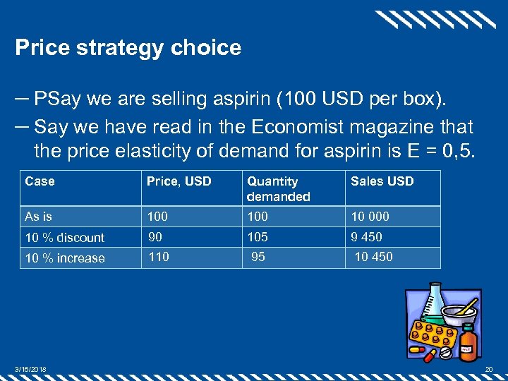Price strategy choice ─ PSay we are selling aspirin (100 USD per box). ─ Say we have read in the Economist magazine that the price elasticity of demand for aspirin is E = 0, 5. Case Price, USD Quantity demanded Sales USD As is 100 10 000 10 % discount 90 105 9 450 10 % increase 110 95 3/16/2018 10 450 20

1. Demand 2. Supply 3. Market equilibrium 3/16/2018 21

Supply ─ the quantities of any particular good which the firms are willing to make available at the variety of prices. 3/16/2018 22

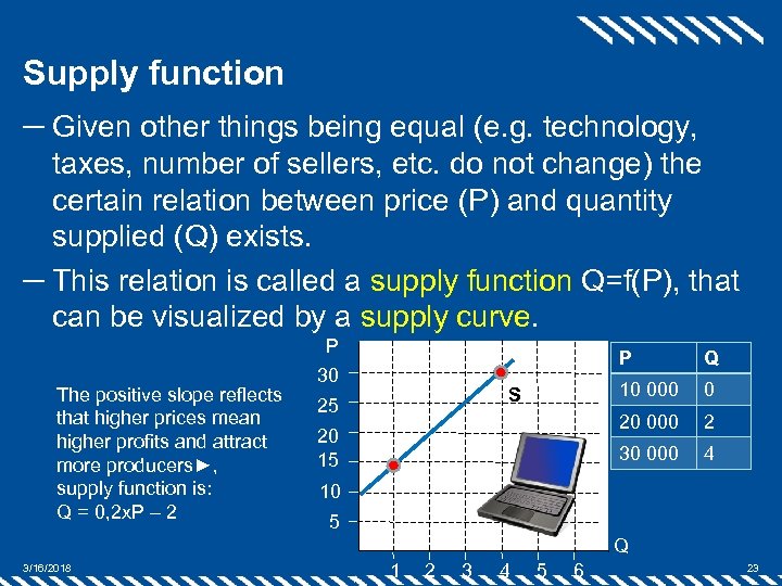Supply function ─ Given other things being equal (e. g. technology, taxes, number of sellers, etc. do not change) the certain relation between price (P) and quantity supplied (Q) exists. ─ This relation is called a supply function Q=f(P), that can be visualized by a supply curve. The positive slope reflects that higher prices mean higher profits and attract more producers►, supply function is: Q = 0, 2 x. P – 2 P 30 P 10 000 2 30 000 20 15 0 20 000 S 25 Q 4 10 5 Q 3/16/2018 1 2 3 4 5 6 23

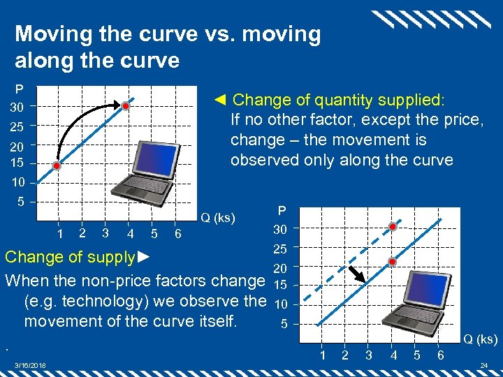Moving the curve vs. moving along the curve P 30 ◄ Change of quantity supplied: If no other factor, except the price, change – the movement is observed only along the curve 25 20 15 10 5 Q (ks) 1 2 3 4 5 6 Change of supply► When the non-price factors change (e. g. technology) we observe the movement of the curve itself. . 3/16/2018 P 30 25 20 15 10 5 Q (ks) 1 2 3 4 5 6 24

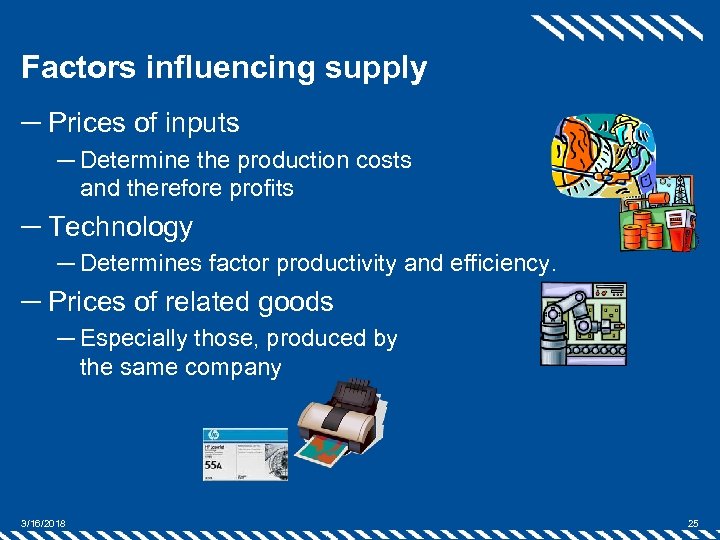Factors influencing supply ─ Prices of inputs ─ Determine the production costs and therefore profits ─ Technology ─ Determines factor productivity and efficiency. ─ Prices of related goods ─ Especially those, produced by the same company 3/16/2018 25

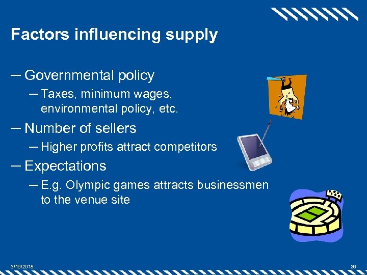Factors influencing supply ─ Governmental policy ─ Taxes, minimum wages, environmental policy, etc. ─ Number of sellers ─ Higher profits attract competitors ─ Expectations ─ E. g. Olympic games attracts businessmen to the venue site 3/16/2018 26

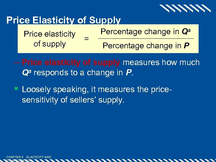Price Elasticity of Supply Price elasticity of supply = Percentage change in Qs Percentage change in P ─ Price elasticity of supply measures how much Qs responds to a change in P. § Loosely speaking, it measures the pricesensitivity of sellers’ supply. CHAPTER 5 ELASTICITY AND ITS APPLICATION

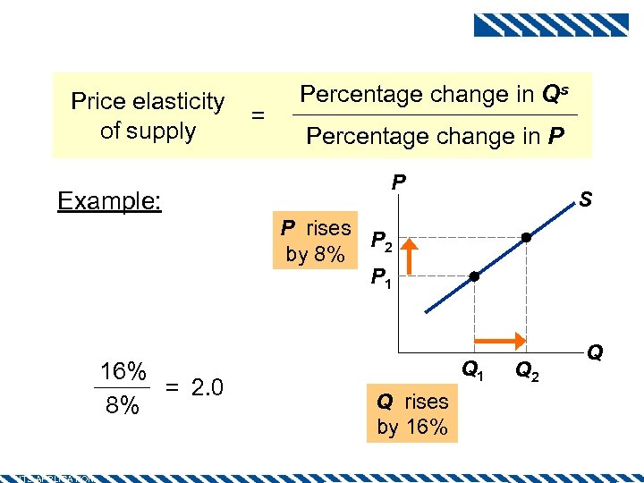Price Elasticity of Supply Price elasticity of supply Example: Price elasticity of supply equals 16% = 2. 0 8% CHAPTER 5 ELASTICITY AND ITS APPLICATION = Percentage change in Qs Percentage change in P P S P rises P 2 by 8% P 1 Q rises by 16% Q 2 Q

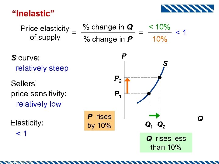“Inelastic” < 10% % change in Q Price elasticity <1 = = of supply 10% % change in P P S curve: relatively steep P 2 Sellers’ price sensitivity: relatively low Elasticity: <1 CHAPTER 5 ELASTICITY AND ITS APPLICATION S P 1 P rises by 10% Q 1 Q 2 Q rises less than 10% Q

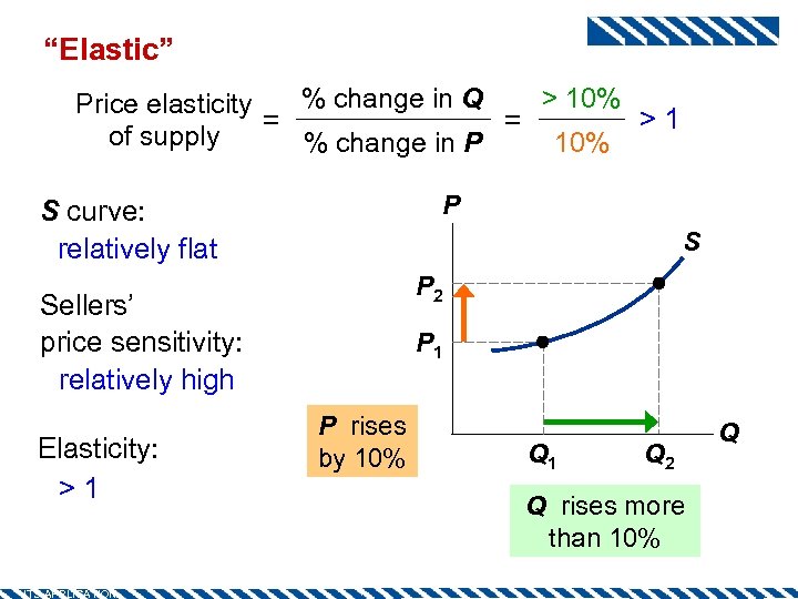“Elastic” > 10% % change in Q Price elasticity >1 = = of supply 10% % change in P P S curve: relatively flat S P 2 Sellers’ price sensitivity: relatively high Elasticity: >1 CHAPTER 5 ELASTICITY AND ITS APPLICATION P 1 P rises by 10% Q 1 Q 2 Q rises more than 10% Q

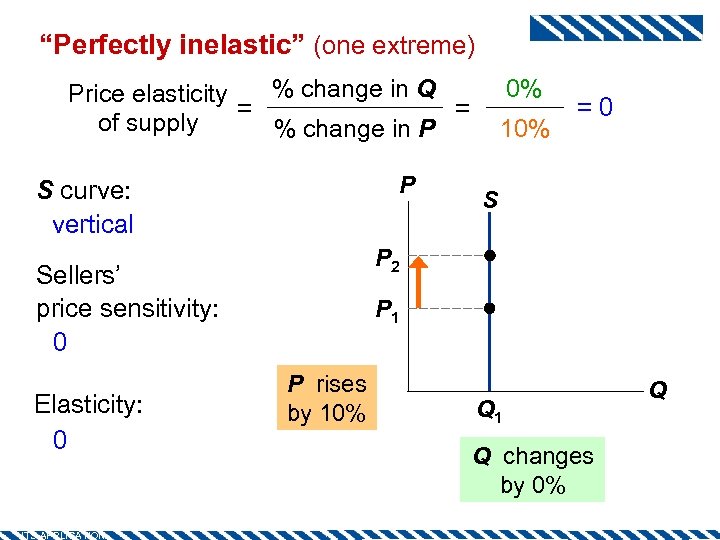“Perfectly inelastic” (one extreme) 0% % change in Q Price elasticity = = of supply % change in P P S curve: vertical CHAPTER 5 ELASTICITY AND ITS APPLICATION S P 2 Sellers’ price sensitivity: 0 Elasticity: 0 10% =0 P 1 P rises by 10% Q 1 Q changes by 0% Q

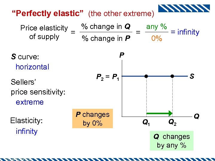“Perfectly elastic” (the other extreme) any % % change in Q Price elasticity = infinity = = of supply 0% % change in P P S curve: horizontal Sellers’ price sensitivity: extreme Elasticity: infinity CHAPTER 5 ELASTICITY AND ITS APPLICATION S P 2 = P 1 P changes by 0% Q 1 Q 2 Q changes by any % Q

The Determinants of Supply Elasticity ─ The more easily sellers can change the quantity they produce, the greater the price elasticity of supply. ─ Example: Supply of beachfront property is harder to vary and thus less elastic than supply of new cars. ─ For many goods, price elasticity of supply is greater in the long run than in the short run, because firms can build new factories, or new firms may be able to enter the market. CHAPTER 5 ELASTICITY AND ITS APPLICATION

1. Demand 2. Supply 3. Market equilibrium 3/16/2018 34

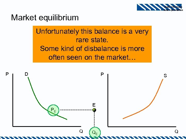Další informace dole v poznámce Market equilibrium Unfortunately this balance is a very … happens when demand equals supply rare state. Some kind of disbalance is more often seen on the market… D P S E PE P Q QE Q

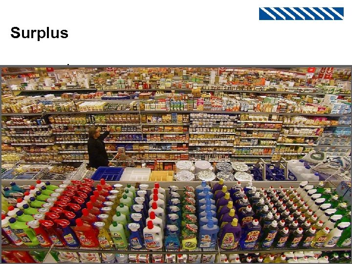Surplus Pi D S P 1 E PE QD =Q E= QS Qi

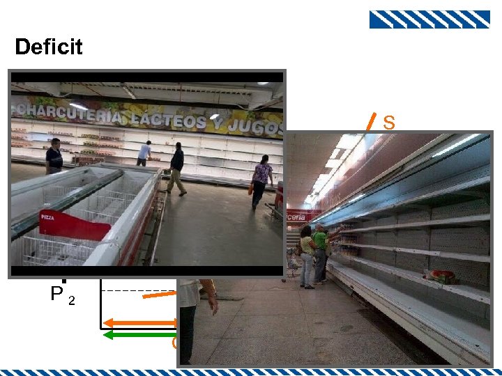Deficit Pi D S E PE P 2 QS =Q E = QD Qi

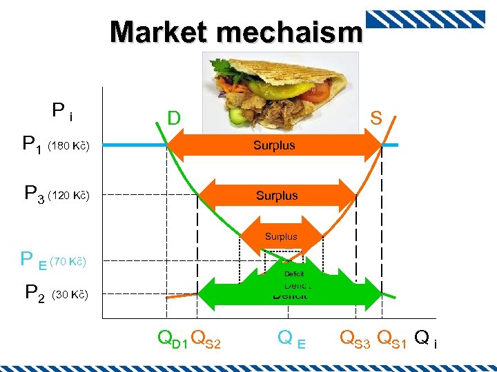Market mechaism Pi D S P 1 (180 Kč) Surplus P 3 (120 Kč) Surplus E P E (70 Kč) P 2 Deficit (30 Kč) QD 1 QS 2 QE QS 3 QS 1 Q i

Utility and consumer behaviour 3/16/2018 39

─ Utility is a measure of the relative satisfaction from consumption of various goods and service. Utility is a subjective feeling when our needs and wants are being satisfied.

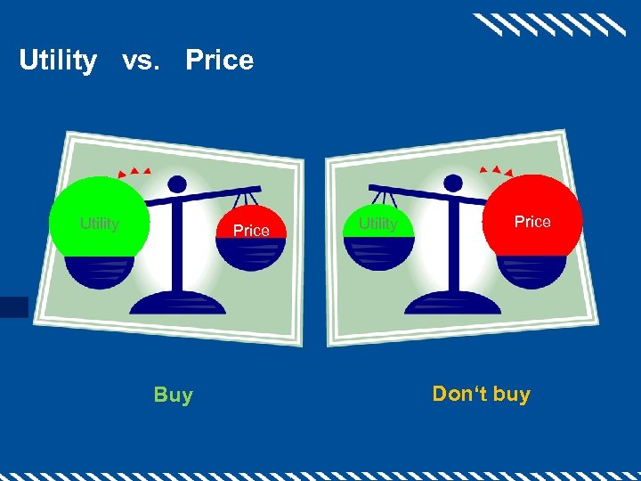Utility vs. Price Utility Price Buy Utility Price Don‘t buy

Can we measure utility? Smartphone Price (standard quality) 25 000 Kč 15 000 Kč 7 000 Kč 2 000 Kč 500 Kč Will you buy it?

Types of utility ─ Total utility (TU) is the utility gained from all consumed goods. n Marginal utility (MU) is the increase of utility by the consumption of another unit of goods („additional“ utility)

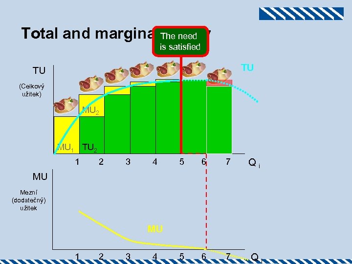Total and marginal The need utiluty is satisfied TU TU (Celkový užitek) MU 2 TU 11 TU 2 MU 1 2 3 4 5 6 7 Qi MU Mezní (dodatečný) užitek MU 1 2 3 4 Qi

Summary ─ We only buy additional unit of the goods when the marginal utility of this unit is higher (or at least at the same level) than its price ─ When we feel that the MU is higher than P – we buy ─ When we feel that the MU is lower than P – we don‘t buy 3/16/2018 45

Thank you for attention!