Introduction to Data Science and Analytics Stephan Sorger

Introduction to Data Science and Analytics Stephan Sorger www. stephansorger. com Unit 5. Excel Forecasting Disclaimer: • All images such as logos, photos, etc. used in this presentation are the property of their respective copyright owners and are used here for educational purposes only • Some material adapted from: Sorger, “Marketing Analytics: Strategic Models and Metrics” © Stephan Sorger 2016; www. stephansorger. com; Data Science: Excel Forecasting

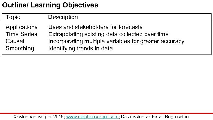Outline/ Learning Objectives Topic Description Applications Time Series Causal Smoothing Uses and stakeholders forecasts Extrapolating existing data collected over time Incorporating multiple variables for greater accuracy Identifying trends in data © Stephan Sorger 2016; www. stephansorger. com; Data Science: Excel Regression

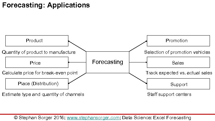Forecasting: Applications Product Promotion Quantity of product to manufacture Price Calculate price for break-even point Place (Distribution) Estimate type and quantity of channels Selection of promotion vehicles Forecasting Sales Track expected vs. actual sales Support Staff support centers © Stephan Sorger 2016; www. stephansorger. com; Data Science: Excel Forecasting

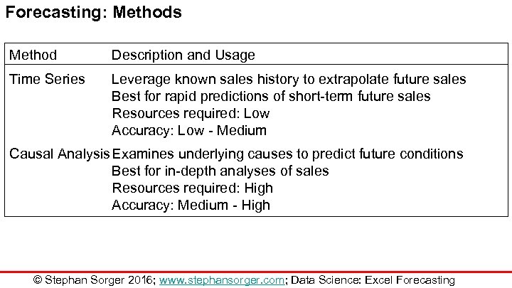Forecasting: Methods Method Description and Usage Time Series Leverage known sales history to extrapolate future sales Best for rapid predictions of short-term future sales Resources required: Low Accuracy: Low - Medium Causal Analysis. Examines underlying causes to predict future conditions Best for in-depth analyses of sales Resources required: High Accuracy: Medium - High © Stephan Sorger 2016; www. stephansorger. com; Data Science: Excel Forecasting

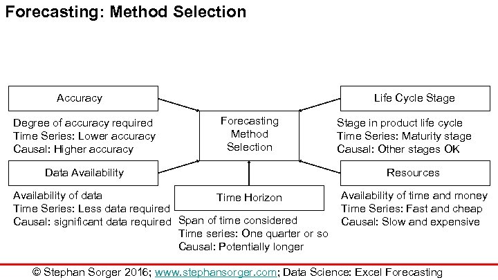Forecasting: Method Selection Accuracy Degree of accuracy required Time Series: Lower accuracy Causal: Higher accuracy Life Cycle Stage Forecasting Method Selection Data Availability of data Time Horizon Time Series: Less data required Causal: significant data required Span of time considered Time series: One quarter or so Causal: Potentially longer Stage in product life cycle Time Series: Maturity stage Causal: Other stages OK Resources Availability of time and money Time Series: Fast and cheap Causal: Slow and expensive © Stephan Sorger 2016; www. stephansorger. com; Data Science: Excel Forecasting

Introduction to Data Science and Analytics Stephan Sorger www. stephansorger. com Unit 5. Excel Forecasting Lecture: Time Series Forecast © Stephan Sorger 2016; www. stephansorger. com; Data Science: Excel Forecasting

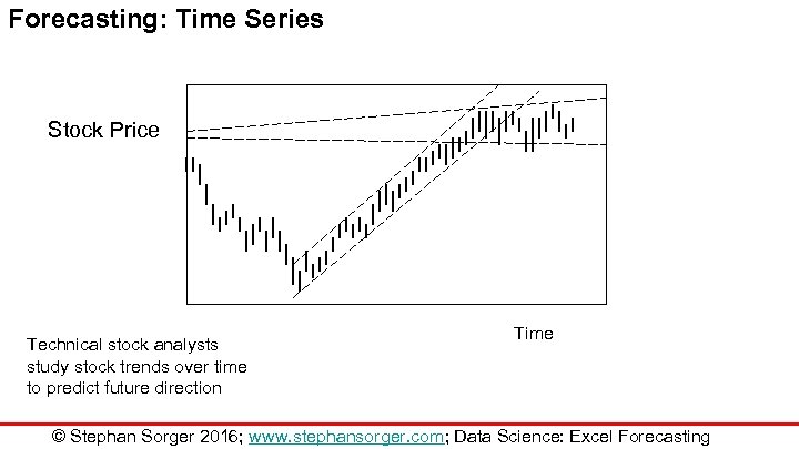Forecasting: Time Series Stock Price Technical stock analysts study stock trends over time to predict future direction Time © Stephan Sorger 2016; www. stephansorger. com; Data Science: Excel Forecasting

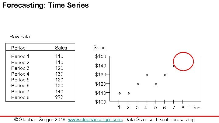Forecasting: Time Series Raw data Period Sales Period 1 Period 2 Period 3 Period 4 Period 5 Period 6 Period 7 Period 8 110 120 130 140 ? ? ? Sales $150 $140 $130 $120 $110 $100 1 2 3 4 5 6 7 8 Time © Stephan Sorger 2016; www. stephansorger. com; Data Science: Excel Forecasting

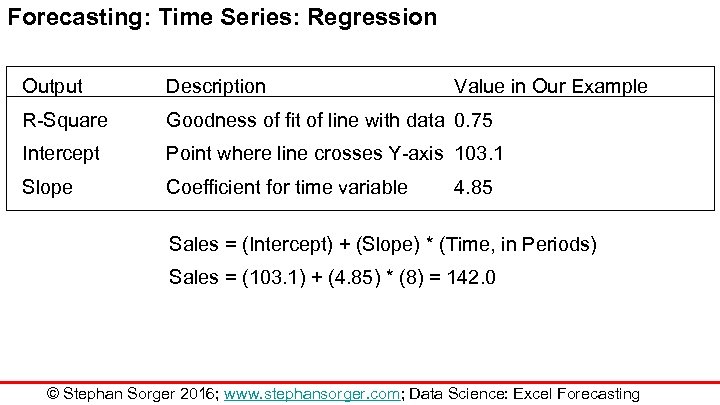Forecasting: Time Series: Regression Output Description Value in Our Example R-Square Goodness of fit of line with data 0. 75 Intercept Point where line crosses Y-axis 103. 1 Slope Coefficient for time variable 4. 85 Sales = (Intercept) + (Slope) * (Time, in Periods) Sales = (103. 1) + (4. 85) * (8) = 142. 0 © Stephan Sorger 2016; www. stephansorger. com; Data Science: Excel Forecasting

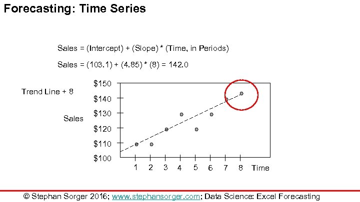Forecasting: Time Series Sales = (Intercept) + (Slope) * (Time, in Periods) Sales = (103. 1) + (4. 85) * (8) = 142. 0 Trend Line + 8 Sales $150 $140 $130 $120 $110 $100 1 2 3 4 5 6 7 8 Time © Stephan Sorger 2016; www. stephansorger. com; Data Science: Excel Forecasting

Introduction to Data Science and Analytics Stephan Sorger www. stephansorger. com Unit 5. Excel Forecasting Lecture: Multivariate Forecast © Stephan Sorger 2016; www. stephansorger. com; Data Science: Excel Forecasting

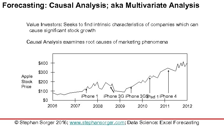Forecasting: Causal Analysis; aka Multivariate Analysis Value Investors: Seeks to find intrinsic characteristics of companies which can cause significant stock growth Causal Analysis examines root causes of marketing phenomena $400 Apple Stock Price $300 $200 $100 $0 2006 i. Phone 1 2007 2008 i. Phone 3 GS i. Pad 1 i. Phone 4 2009 2010 2011 2012 © Stephan Sorger 2016; www. stephansorger. com; Data Science: Excel Forecasting

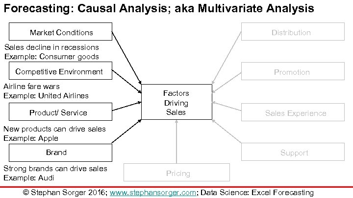Forecasting: Causal Analysis; aka Multivariate Analysis Market Conditions Distribution Sales decline in recessions Example: Consumer goods Competitive Environment Airline fare wars Example: United Airlines Product/ Service Promotion Factors Driving Sales Experience New products can drive sales Example: Apple Brand Strong brands can drive sales Example: Audi Support Pricing © Stephan Sorger 2016; www. stephansorger. com; Data Science: Excel Forecasting

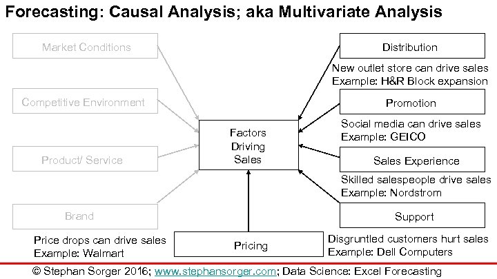Forecasting: Causal Analysis; aka Multivariate Analysis Distribution Market Conditions New outlet store can drive sales Example: H&R Block expansion Competitive Environment Product/ Service Promotion Factors Driving Sales Social media can drive sales Example: GEICO Sales Experience Skilled salespeople drive sales Example: Nordstrom Brand Price drops can drive sales Example: Walmart Support Pricing Disgruntled customers hurt sales Example: Dell Computers © Stephan Sorger 2016; www. stephansorger. com; Data Science: Excel Forecasting

Introduction to Data Science and Analytics Stephan Sorger www. stephansorger. com Unit 5. Excel Forecasting Lecture: Forecasting Example © Stephan Sorger 2016; www. stephansorger. com; Data Science: Excel Forecasting

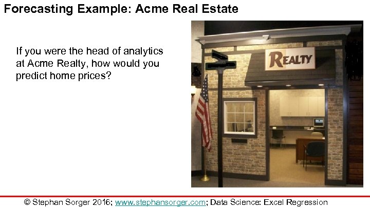Forecasting Example: Acme Real Estate If you were the head of analytics at Acme Realty, how would you predict home prices? © Stephan Sorger 2016; www. stephansorger. com; Data Science: Excel Regression

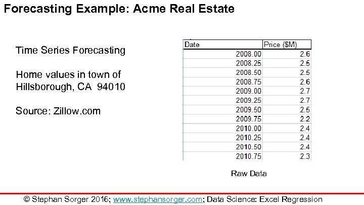Forecasting Example: Acme Real Estate Time Series Forecasting Home values in town of Hillsborough, CA 94010 Source: Zillow. com Raw Data © Stephan Sorger 2016; www. stephansorger. com; Data Science: Excel Regression

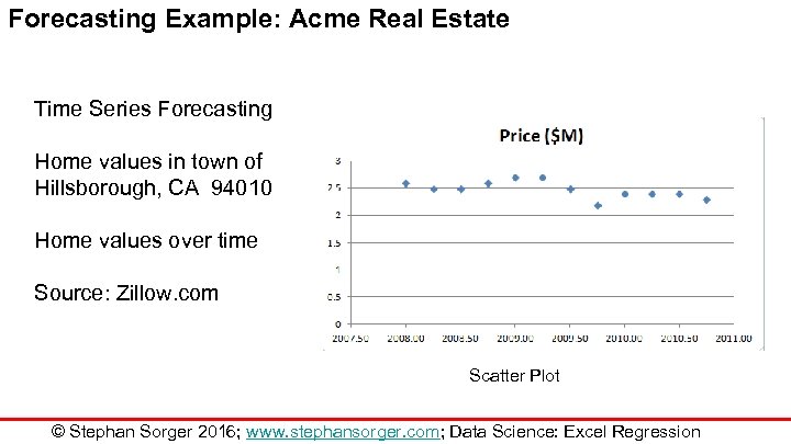Forecasting Example: Acme Real Estate Time Series Forecasting Home values in town of Hillsborough, CA 94010 Home values over time Source: Zillow. com Scatter Plot © Stephan Sorger 2016; www. stephansorger. com; Data Science: Excel Regression

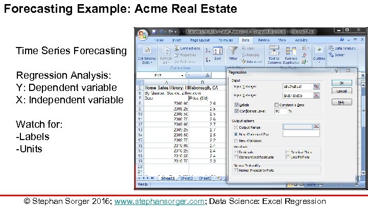Forecasting Example: Acme Real Estate Time Series Forecasting Regression Analysis: Y: Dependent variable X: Independent variable Watch for: -Labels -Units © Stephan Sorger 2016; www. stephansorger. com; Data Science: Excel Regression

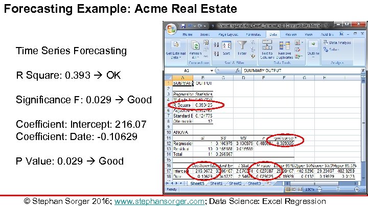Forecasting Example: Acme Real Estate Time Series Forecasting R Square: 0. 393 OK Significance F: 0. 029 Good Coefficient: Intercept: 216. 07 Coefficient: Date: -0. 10629 P Value: 0. 029 Good © Stephan Sorger 2016; www. stephansorger. com; Data Science: Excel Regression

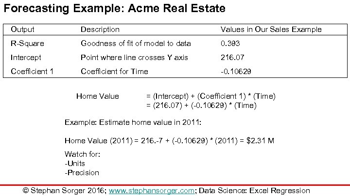Forecasting Example: Acme Real Estate Output Description Values in Our Sales Example R-Square Goodness of fit of model to data 0. 393 Intercept Point where line crosses Y axis 216. 07 Coefficient 1 Coefficient for Time -0. 10629 Home Value = (Intercept) + (Coefficient 1) * (Time) = (216. 07) + (-0. 10629) * (Time) Example: Estimate home value in 2011: Home Value (2011) = 216. -7 + (-0. 10629) * (2011) = $2. 31 M Watch for: -Units -Precision © Stephan Sorger 2016; www. stephansorger. com; Data Science: Excel Regression

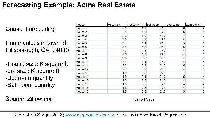Forecasting Example: Acme Real Estate Causal Forecasting Home values in town of Hillsborough, CA 94010 -House size: K square ft -Lot size: K square ft -Bedroom quantity -Bathroom quantity Source: Zillow. com Raw Data © Stephan Sorger 2016; www. stephansorger. com; Data Science: Excel Regression

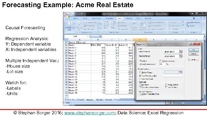Forecasting Example: Acme Real Estate Causal Forecasting Regression Analysis: Y: Dependent variable X: Independent variables Multiple Independent Var. : -House size -Lot size Watch for: -Labels -Units © Stephan Sorger 2016; www. stephansorger. com; Data Science: Excel Regression

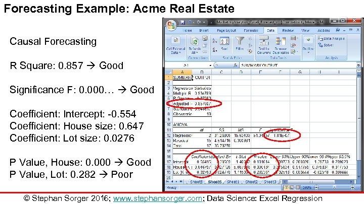Forecasting Example: Acme Real Estate Causal Forecasting R Square: 0. 857 Good Significance F: 0. 000… Good Coefficient: Intercept: -0. 554 Coefficient: House size: 0. 647 Coefficient: Lot size: 0. 0276 P Value, House: 0. 000 Good P Value, Lot: 0. 282 Poor © Stephan Sorger 2016; www. stephansorger. com; Data Science: Excel Regression

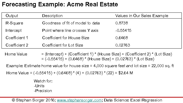Forecasting Example: Acme Real Estate Output Description Values in Our Sales Example R-Square Goodness of fit of model to data 0. 8738 Intercept Point where line crosses Y axis -0. 55415 Coefficient 1 Coefficient for House Size 0. 6468 Coefficient 2 Coefficient for Lot Size 0. 02763 Home Value = (Intercept) + (Coefficient 1) * (House Size) + (Coefficient 2) * (Lot Size) = (-0. 55415) + (0. 6468) * (House Size) + (0. 02763) * (Lot Size) Example: Estimate home value for house size = 4, 000 square feet and lot size = 22, 000 sq. ft Home Value = (-0. 55415) + (0. 6468) * (4) + (0. 02763) * (22) = $2. 64 M Watch for: -Units -Precision © Stephan Sorger 2016; www. stephansorger. com; Data Science: Excel Regression

Introduction to Data Science and Analytics Stephan Sorger www. stephansorger. com Unit 5. Excel Forecasting Lecture: Smoothing © Stephan Sorger 2016; www. stephansorger. com; Data Science: Excel Forecasting

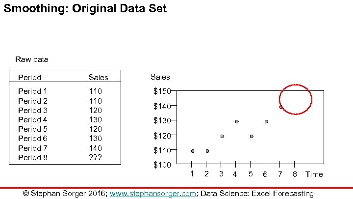Smoothing: Original Data Set Raw data Period Sales Period 1 Period 2 Period 3 Period 4 Period 5 Period 6 Period 7 Period 8 110 120 130 140 ? ? ? Sales $150 $140 $130 $120 $110 $100 1 2 3 4 5 6 7 8 Time © Stephan Sorger 2016; www. stephansorger. com; Data Science: Excel Forecasting

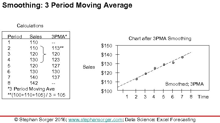Smoothing: 3 Period Moving Average Calculations Period Sales 3 PMA* 1 110 -2 110 113** 3 120 4 130 123 5 120 127 6 130 7 140 137 8 142 -*3 Period Moving Ave **(100+110+105) / 3 = 105 Chart after 3 PMA Smoothing $150 $140 Sales $130 $120 $110 Smoothed; 3 PMA $100 1 2 3 4 5 6 7 8 © Stephan Sorger 2016; www. stephansorger. com; Data Science: Excel Forecasting Time

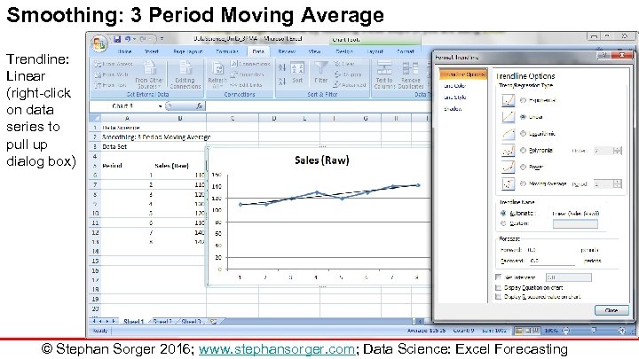Smoothing: 3 Period Moving Average Trendline: Linear (right-click on data series to pull up dialog box) © Stephan Sorger 2016; www. stephansorger. com; Data Science: Excel Forecasting

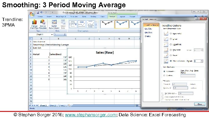Smoothing: 3 Period Moving Average Trendline: 3 PMA © Stephan Sorger 2016; www. stephansorger. com; Data Science: Excel Forecasting

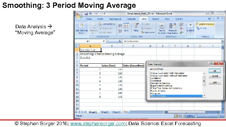Smoothing: 3 Period Moving Average Data Analysis “Moving Average” © Stephan Sorger 2016; www. stephansorger. com; Data Science: Excel Forecasting

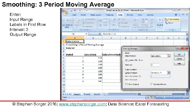Smoothing: 3 Period Moving Average Enter: Input Range Labels in First Row Interval: 3 Output Range © Stephan Sorger 2016; www. stephansorger. com; Data Science: Excel Forecasting

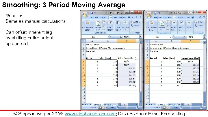Smoothing: 3 Period Moving Average Results: Same as manual calculations Can offset inherent lag by shifting entire output up one cell © Stephan Sorger 2016; www. stephansorger. com; Data Science: Excel Forecasting

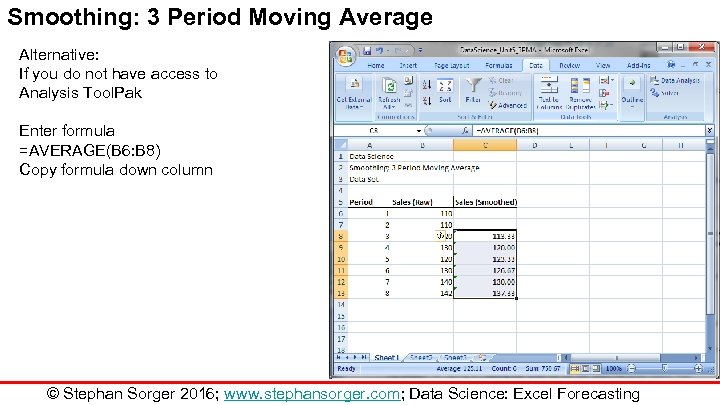Smoothing: 3 Period Moving Average Alternative: If you do not have access to Analysis Tool. Pak Enter formula =AVERAGE(B 6: B 8) Copy formula down column © Stephan Sorger 2016; www. stephansorger. com; Data Science: Excel Forecasting

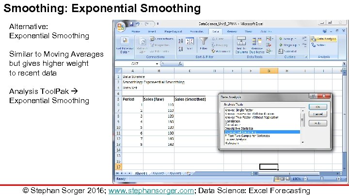Smoothing: Exponential Smoothing Alternative: Exponential Smoothing Similar to Moving Averages but gives higher weight to recent data Analysis Tool. Pak Exponential Smoothing © Stephan Sorger 2016; www. stephansorger. com; Data Science: Excel Forecasting

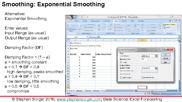Smoothing: Exponential Smoothing Alternative: Exponential Smoothing Enter values: Input Range (as usual) Output Range (as usual) Damping Factor (DF) Damping Factor = (1 – a) a = smoothing constant a = 0. 1 DF = 0. 9 high damping, peaks smoothed a = 0. 9 DF = 0. 1 low damping, little smoothing a = 0. 5 DF = 0. 5 compromise © Stephan Sorger 2016; www. stephansorger. com; Data Science: Excel Forecasting

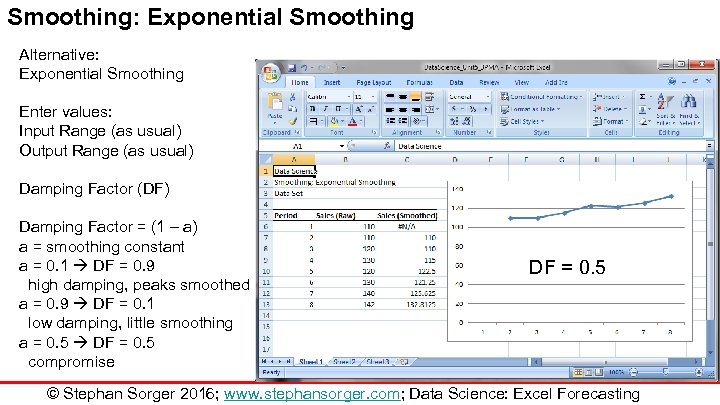Smoothing: Exponential Smoothing Alternative: Exponential Smoothing Enter values: Input Range (as usual) Output Range (as usual) Damping Factor (DF) Damping Factor = (1 – a) a = smoothing constant a = 0. 1 DF = 0. 9 high damping, peaks smoothed a = 0. 9 DF = 0. 1 low damping, little smoothing a = 0. 5 DF = 0. 5 compromise DF = 0. 5 © Stephan Sorger 2016; www. stephansorger. com; Data Science: Excel Forecasting

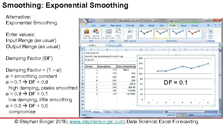Smoothing: Exponential Smoothing Alternative: Exponential Smoothing Enter values: Input Range (as usual) Output Range (as usual) Damping Factor (DF) Damping Factor = (1 – a) a = smoothing constant a = 0. 1 DF = 0. 9 high damping, peaks smoothed a = 0. 9 DF = 0. 1 low damping, little smoothing a = 0. 5 DF = 0. 5 compromise DF = 0. 1 © Stephan Sorger 2016; www. stephansorger. com; Data Science: Excel Forecasting

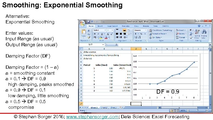Smoothing: Exponential Smoothing Alternative: Exponential Smoothing Enter values: Input Range (as usual) Output Range (as usual) Damping Factor (DF) Damping Factor = (1 – a) a = smoothing constant a = 0. 1 DF = 0. 9 high damping, peaks smoothed a = 0. 9 DF = 0. 1 low damping, little smoothing a = 0. 5 DF = 0. 5 compromise DF = 0. 9 © Stephan Sorger 2016; www. stephansorger. com; Data Science: Excel Forecasting

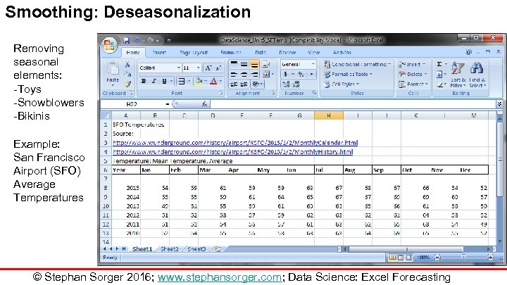Smoothing: Deseasonalization Removing seasonal elements: -Toys -Snowblowers -Bikinis Example: San Francisco Airport (SFO) Average Temperatures © Stephan Sorger 2016; www. stephansorger. com; Data Science: Excel Forecasting

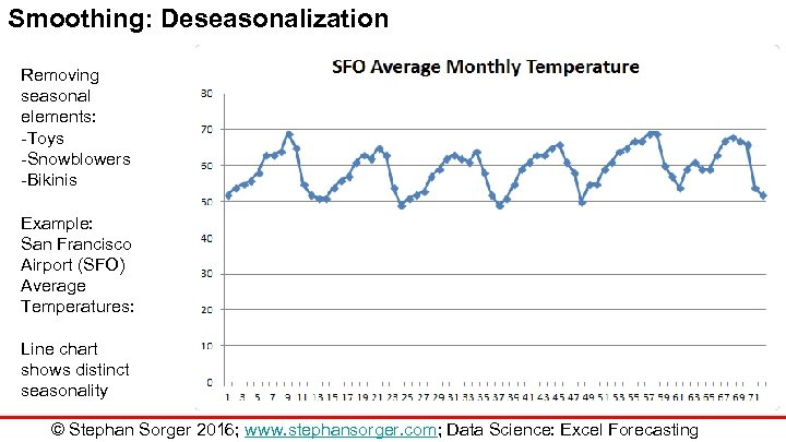Smoothing: Deseasonalization Removing seasonal elements: -Toys -Snowblowers -Bikinis Example: San Francisco Airport (SFO) Average Temperatures: Line chart shows distinct seasonality © Stephan Sorger 2016; www. stephansorger. com; Data Science: Excel Forecasting

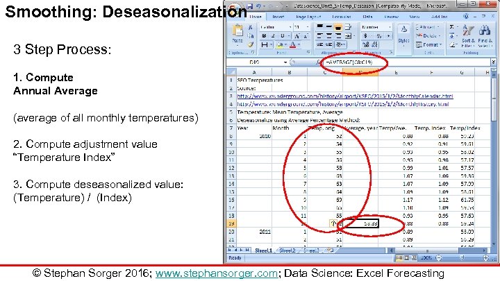Smoothing: Deseasonalization 3 Step Process: 1. Compute Annual Average (average of all monthly temperatures) 2. Compute adjustment value “Temperature Index” 3. Compute deseasonalized value: (Temperature) / (Index) © Stephan Sorger 2016; www. stephansorger. com; Data Science: Excel Forecasting

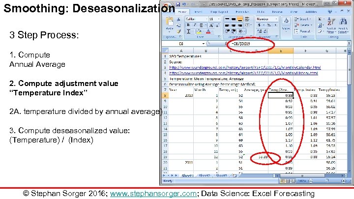Smoothing: Deseasonalization 3 Step Process: 1. Compute Annual Average 2. Compute adjustment value “Temperature Index” 2 A. temperature divided by annual average) 3. Compute deseasonalized value: (Temperature) / (Index) © Stephan Sorger 2016; www. stephansorger. com; Data Science: Excel Forecasting

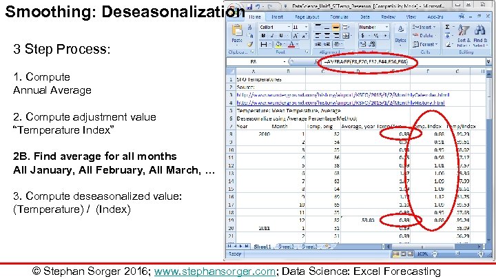Smoothing: Deseasonalization 3 Step Process: 1. Compute Annual Average 2. Compute adjustment value “Temperature Index” 2 B. Find average for all months All January, All February, All March, … 3. Compute deseasonalized value: (Temperature) / (Index) © Stephan Sorger 2016; www. stephansorger. com; Data Science: Excel Forecasting

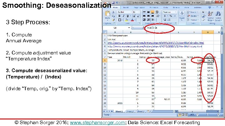Smoothing: Deseasonalization 3 Step Process: 1. Compute Annual Average 2. Compute adjustment value “Temperature Index” 3. Compute deseasonalized value: (Temperature) / (Index) (divide “Temp, orig. ” by “Temp. Index”) © Stephan Sorger 2016; www. stephansorger. com; Data Science: Excel Forecasting

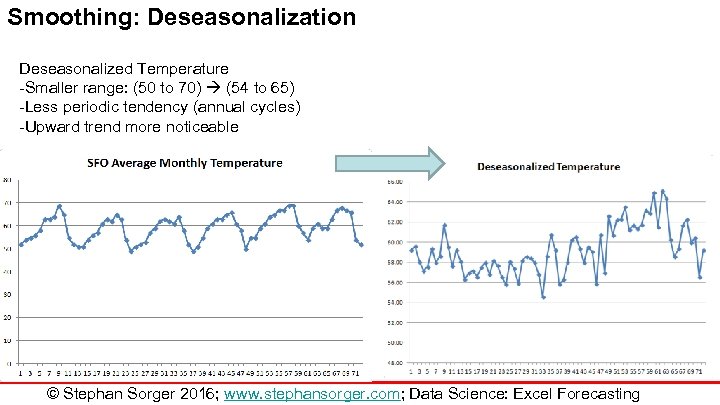Smoothing: Deseasonalization Deseasonalized Temperature -Smaller range: (50 to 70) (54 to 65) -Less periodic tendency (annual cycles) -Upward trend more noticeable © Stephan Sorger 2016; www. stephansorger. com; Data Science: Excel Forecasting

Outline/ Learning Objectives Topic Description Applications Time Series Causal Smoothing Uses and stakeholders forecasts Extrapolating existing data collected over time Incorporating multiple variables for greater accuracy Identifying trends in data © Stephan Sorger 2016; www. stephansorger. com; Data Science: Excel Regression