Introduction to Data Mining Association Rules Reference Tan

Introduction to Data Mining Association Rules Reference: Tan et al: Introduction to data mining. Some slides are adopted from Tan et al

What is Data Mining? Data mining is the exploration and analysis of large quantities of data in order to discover valid, novel, potentially useful, and ultimately understandable patterns in data.

What is data mining (cont. )? Valid: The patterns hold in general. Novel: We did not know the pattern beforehand. Useful: We can devise actions from the patterns. Understandable: We can interpret and comprehend the patterns. Data mining falls into the broad field of knowledge discovery

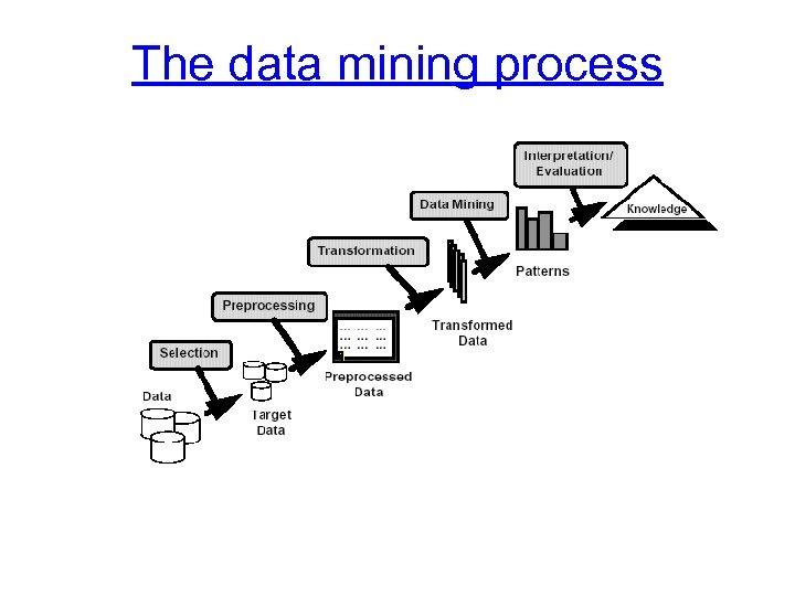The data mining process

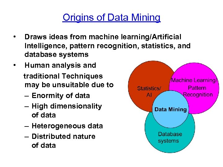Origins of Data Mining • • Draws ideas from machine learning/Artificial Intelligence, pattern recognition, statistics, and database systems Human analysis and traditional Techniques may be unsuitable due to Statistics/ AI – Enormity of data – High dimensionality of data – Heterogeneous data – Distributed nature of data

Data Mining Tasks • Prediction Methods – Use some variables to predict unknown or future values of other variables. • Description Methods – Find human-interpretable patterns that describe the data.

Data Mining Tasks. . . • • • Association Rule Discovery [Descriptive] Clustering [Descriptive] Classification [Predictive] (for discrete variables) Sequential Pattern Discovery [Descriptive] Regression [Predictive] (for continuous variable) Deviation Detection [Predictive]

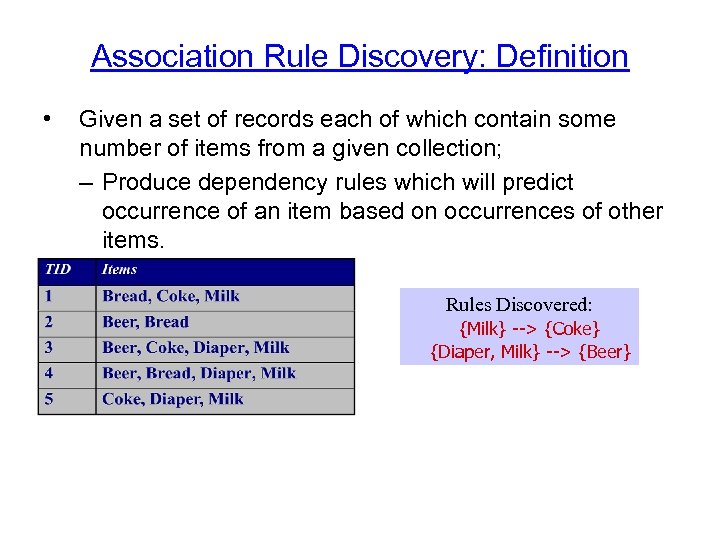Association Rule Discovery: Definition • Given a set of records each of which contain some number of items from a given collection; – Produce dependency rules which will predict occurrence of an item based on occurrences of other items. Rules Discovered: {Milk} --> {Coke} {Diaper, Milk} --> {Beer}

Association Rule Discovery: Sample Application • Supermarket shelf management. – Goal: To identify items that are bought together by sufficiently many customers. – Approach: Process the point-of-sale data collected with barcode scanners to find dependencies among items.

Clustering: Definition Given a set of data points, each having a set of attributes, and a similarity measure among them, find clusters such that – Data points in one cluster are more similar to one another. – Data points in separate clusters are less similar to one another. Similarity Measures: – Euclidean Distance if attributes are continuous. – Other Problem-specific Measures.

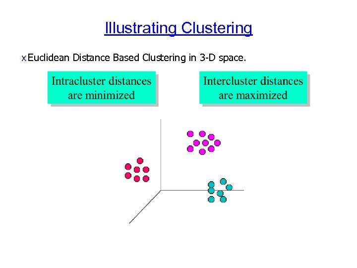Illustrating Clustering x Euclidean Distance Based Clustering in 3 -D space.

Clustering: Sample Application 1 Market Segmentation: – Goal: subdivide a market into distinct subsets of customers where any subset may conceivably be selected as a market target to be reached with a distinct marketing mix. – Approach: • Collect different attributes of customers based on their geographical and lifestyle related information. • Find clusters of similar customers. • Measure the clustering quality by observing buying patterns of customers in same cluster vs. those from different clusters.

Clustering: sample application 2 • Document Clustering: – Goal: To find groups of documents that are similar to each other based on the important terms appearing in them. – Approach: To identify frequently occurring terms in each document. Form a similarity measure based on the frequencies of different terms. Use it to cluster. – Gain: Information Retrieval can utilize the clusters to relate a new document or search term to clustered documents.

Classification: Definition Given a collection of records (training set ) – Each record contains a set of attributes, one of the attributes is the class. Find a model for class attribute as a function of the values of other attributes. Goal: previously unseen records should be assigned a class as accurately as possible. – A test set is used to determine the accuracy of the model. Usually, the given data set is divided into training and test sets, with training set used to build the model and test set used to validate it.

Classification and Clustering • Classification: – Classes pre-defined – Uses training set (thus also known as supervised learning) • Clustering: – Classes not defined in advance – No training set (thus also known as unsupervised learning)

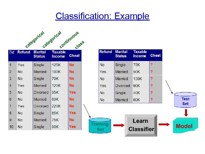Classification: Example

Classification: sample application 1 • Direct Marketing – Goal: Reduce cost of mailing by targeting a set of consumers likely to buy a new cell-phone product. – Approach: • Use the data for a similar product introduced before. • We know which customers decided to buy and which decided otherwise. This {buy, don’t buy} decision forms the class attribute. • Collect various demographic, lifestyle, and companyinteraction related information about all such customers. – Type of business, where they stay, how much they earn, etc. • Use this information as input attributes to learn a classifier model.

Classification: sample application 2 Fraud Detection – Goal: Predict fraudulent cases in credit card transactions. – Approach: • Use credit card transactions and the information on its account-holder as attributes. – When does a customer buy, what does he buy, how often he pays on time, etc • Label past transactions as fraud or fair transactions. This forms the class attribute. • Learn a model for the class of the transactions. • Use this model to detect fraud by observing credit card transactions on an account.

Sequential Pattern Discovery: Definition Given a set of objects, with each object associated with its own timeline of events, find rules that predict strong sequential dependencies among different events. Rules are formed by first discovering patterns. Event occurrences in the patterns are governed by timing constraints.

Regression • Predict a value of a given continuous valued variable based on the values of other variables, assuming a linear or nonlinear model of dependency. • Greatly studied in statistics, neural network fields. • Examples: – Predicting sales amounts of new product based on advetising expenditure. – Predicting wind velocities as a function of temperature, humidity, air pressure, etc. – Time series prediction of stock market indices.

Deviation/Anomaly Detection • Detect significant deviations from normal behavior • Applications: – Credit Card Fraud Detection – Network Intrusion Detection

Mining Association Rules

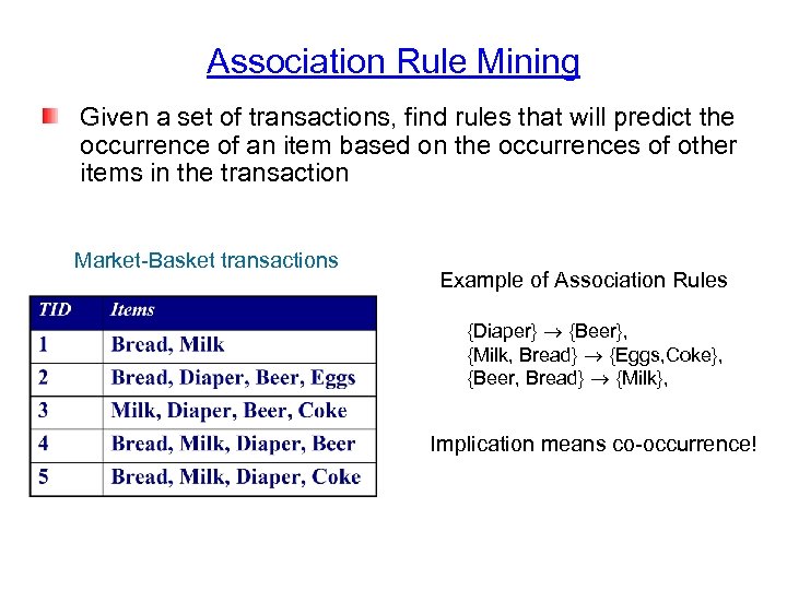Association Rule Mining Given a set of transactions, find rules that will predict the occurrence of an item based on the occurrences of other items in the transaction Market-Basket transactions Example of Association Rules {Diaper} {Beer}, {Milk, Bread} {Eggs, Coke}, {Beer, Bread} {Milk}, Implication means co-occurrence!

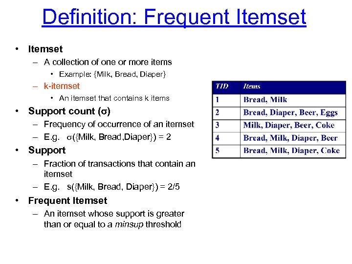Definition: Frequent Itemset • Itemset – A collection of one or more items • Example: {Milk, Bread, Diaper} – k-itemset • An itemset that contains k items • Support count ( ) – Frequency of occurrence of an itemset – E. g. ({Milk, Bread, Diaper}) = 2 • Support – Fraction of transactions that contain an itemset – E. g. s({Milk, Bread, Diaper}) = 2/5 • Frequent Itemset – An itemset whose support is greater than or equal to a minsup threshold

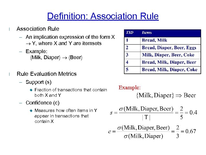Definition: Association Rule l Association Rule – An implication expression of the form X Y, where X and Y are itemsets – Example: {Milk, Diaper} {Beer} l Rule Evaluation Metrics – Support (s) u Fraction of transactions that contain both X and Y – Confidence (c) u Measures how often items in Y appear in transactions that contain X Example:

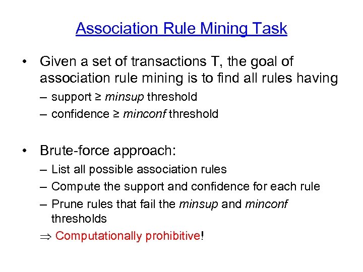Association Rule Mining Task • Given a set of transactions T, the goal of association rule mining is to find all rules having – support ≥ minsup threshold – confidence ≥ minconf threshold • Brute-force approach: – List all possible association rules – Compute the support and confidence for each rule – Prune rules that fail the minsup and minconf thresholds Computationally prohibitive!

Mining Association Rules Example of Rules: {Milk, Diaper} {Beer} (s=0. 4, c=0. 67) {Milk, Beer} {Diaper} (s=0. 4, c=1. 0) {Diaper, Beer} {Milk} (s=0. 4, c=0. 67) {Beer} {Milk, Diaper} (s=0. 4, c=0. 67) {Diaper} {Milk, Beer} (s=0. 4, c=0. 5) {Milk} {Diaper, Beer} (s=0. 4, c=0. 5) Observations: • All the above rules are binary partitions of the same itemset: {Milk, Diaper, Beer} • Rules originating from the same itemset have identical support but can have different confidence • Thus, we may decouple the support and confidence requirements

Mining Association Rules • Two-step approach: 1. Frequent Itemset Generation – Generate all itemsets whose support minsup 2. Rule Generation – Generate high confidence rules from each frequent itemset, where each rule is a binary partitioning of a frequent itemset • Frequent itemset generation is still computationally expensive

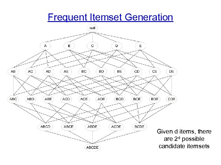Frequent Itemset Generation Given d items, there are 2 d possible candidate itemsets

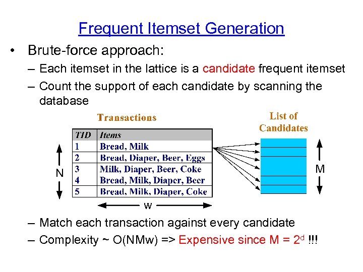Frequent Itemset Generation • Brute-force approach: – Each itemset in the lattice is a candidate frequent itemset – Count the support of each candidate by scanning the database – Match each transaction against every candidate – Complexity ~ O(NMw) => Expensive since M = 2 d !!!

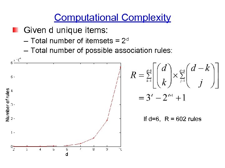Computational Complexity Given d unique items: – Total number of itemsets = 2 d – Total number of possible association rules: If d=6, R = 602 rules

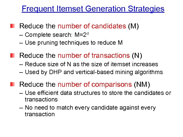Frequent Itemset Generation Strategies Reduce the number of candidates (M) – Complete search: M=2 d – Use pruning techniques to reduce M Reduce the number of transactions (N) – Reduce size of N as the size of itemset increases – Used by DHP and vertical-based mining algorithms Reduce the number of comparisons (NM) – Use efficient data structures to store the candidates or transactions – No need to match every candidate against every transaction

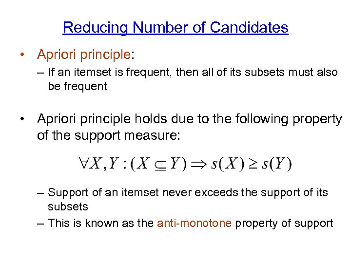Reducing Number of Candidates • Apriori principle: – If an itemset is frequent, then all of its subsets must also be frequent • Apriori principle holds due to the following property of the support measure: – Support of an itemset never exceeds the support of its subsets – This is known as the anti-monotone property of support

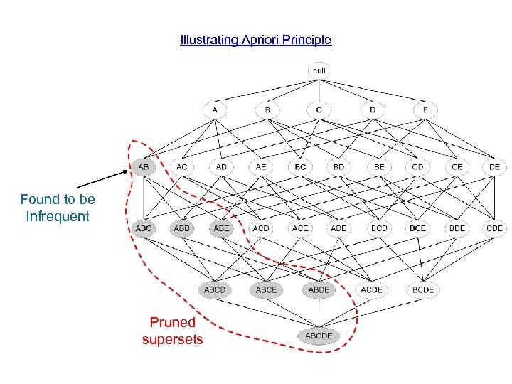Illustrating Apriori Principle Found to be Infrequent Pruned supersets

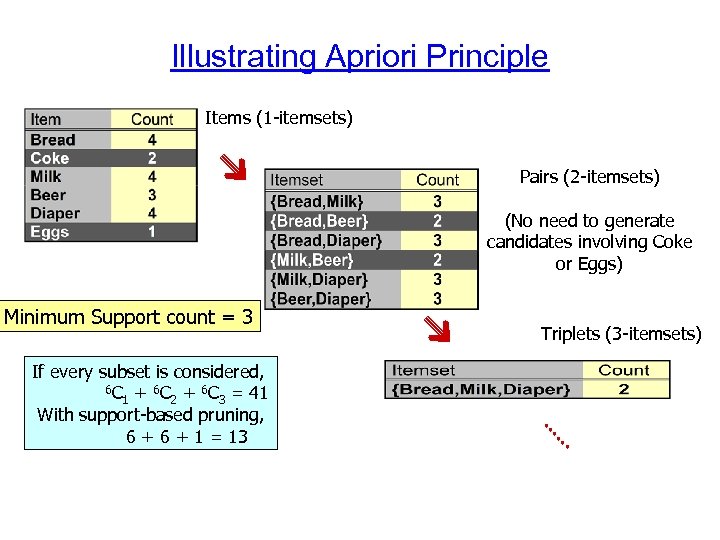Illustrating Apriori Principle Items (1 -itemsets) Pairs (2 -itemsets) (No need to generate candidates involving Coke or Eggs) Minimum Support count = 3 If every subset is considered, 6 C + 6 C = 41 1 2 3 With support-based pruning, 6 + 1 = 13 Triplets (3 -itemsets)

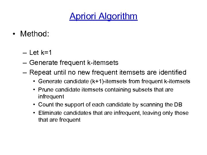Apriori Algorithm • Method: – Let k=1 – Generate frequent k-itemsets – Repeat until no new frequent itemsets are identified • Generate candidate (k+1)-itemsets from frequent k-itemsets • Prune candidate itemsets containing subsets that are infrequent • Count the support of each candidate by scanning the DB • Eliminate candidates that are infrequent, leaving only those that are frequent

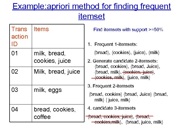Example: apriori method for finding frequent itemset Trans Items action ID 01 02 milk, bread, cookies, juice Milk, bread, juice 03 milk, eggs 04 bread, cookies, coffee Find itemsets with support >=50% 1. Frequent 1 -itemsets: {bread}, {cookies}, {juice}, {milk} 2. Generate candidate 2 -itemsets: {bread, cookies}, {bread, Juice}, {bread, milk}, {cookies, juice}, {cookies, milk}, {juice, milk} 3. Frequent 2 -itemsets {bread, cookies} {bread, Juice} {bread, milk} { juice, milk} 4. candidate 3 -itemsets {bread, cookies, juice}, {bread, cookies, milk}, {bread, juice, milk}

Counting the support counting: – Scan the database of transactions to determine the support of each candidate itemset – To reduce the number of comparisons, store the candidates in a hash structure • Instead of matching each transaction against every candidate, match it against candidates contained in the hashed buckets (details omitted)

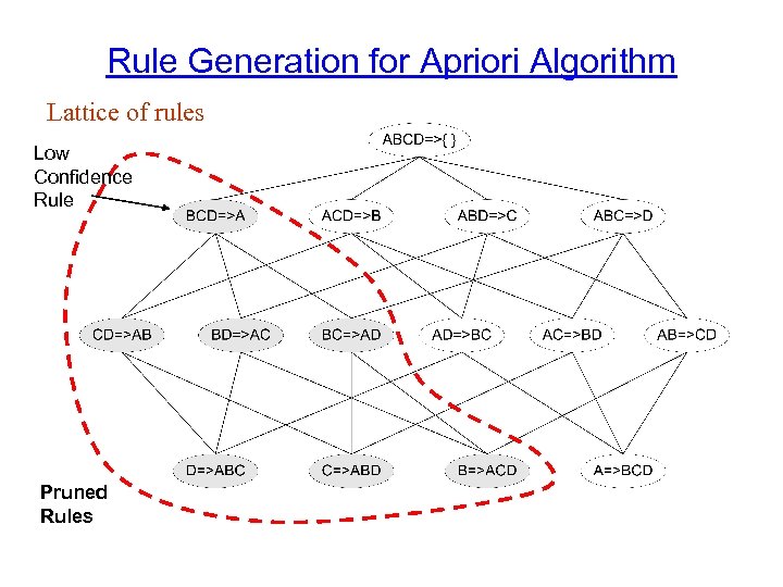Rule Generation for Apriori Algorithm Lattice of rules Low Confidence Rule Pruned Rules

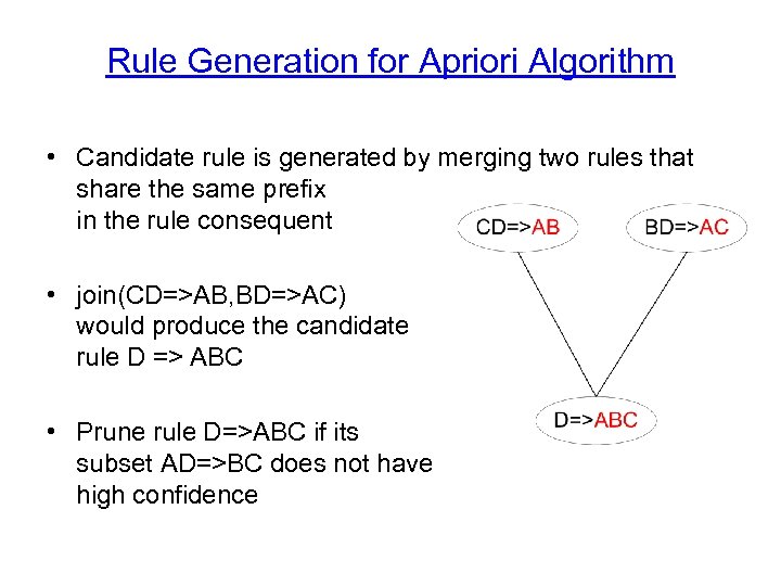Rule Generation for Apriori Algorithm • Candidate rule is generated by merging two rules that share the same prefix in the rule consequent • join(CD=>AB, BD=>AC) would produce the candidate rule D => ABC • Prune rule D=>ABC if its subset AD=>BC does not have high confidence

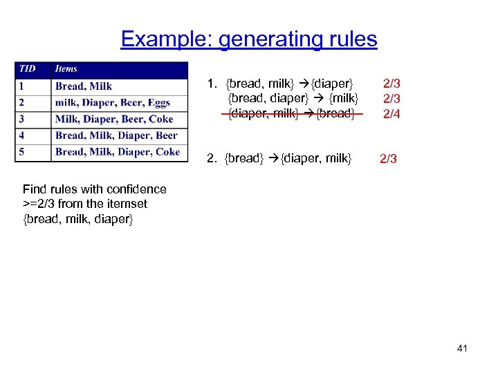Example: generating rules 1. {bread, milk} {diaper} {bread, diaper} {milk} {diaper, milk} {bread} 2. {bread} {diaper, milk} 2/3 2/4 2/3 Find rules with confidence >=2/3 from the itemset {bread, milk, diaper} 41

Next • Clustering • classification 42