8b425c6ffd92a3075a321596ddcc5622.ppt
- Количество слайдов: 28

Introduction to Business Strategy Prof. Marvin Lieberman UCLA Anderson School of Management How Competition Shapes the Creation and Distribution of Economic Value Lecture 3: Competitive Advantage © 2009 by Marvin Lieberman

Competitive Advantage In the previous lecture, we considered how Porter's “five forces” operate at the level of an industry. In this lecture, we look within an industry and consider how differences among firms – and potentially among their customers – give rise to “competitive advantage. ” © 2009 by Marvin Lieberman

Porter (1980) proposed that there are two types of “competitive advantage” • Cost Advantage • Differentiation Advantage Experts in business strategy hold differing views about the exact nature and sources of competitive advantage. Most would agree, however, that competitive advantage must be based on cost or differentiation factors. Let’s start by considering cost advantage. *Michael E. Porter (1980). Competitive Strategy. Free Press, Boston.
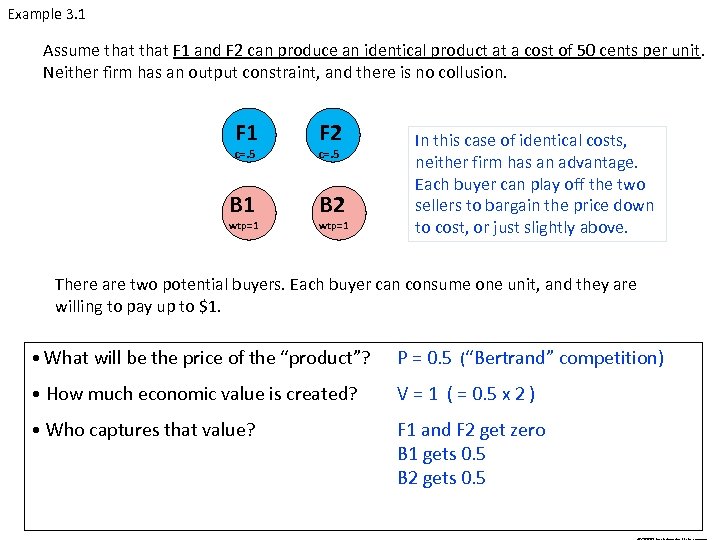
Example 3. 1 Assume that F 1 and F 2 can produce an identical product at a cost of 50 cents per unit. Neither firm has an output constraint, and there is no collusion. F 1 F 2 B 1 B 2 c=. 5 wtp=1 In this case of identical costs, neither firm has an advantage. Each buyer can play off the two sellers to bargain the price down to cost, or just slightly above. There are two potential buyers. Each buyer can consume one unit, and they are willing to pay up to $1. • What will be the price of the “product”? P = 0. 5 (“Bertrand” competition) • How much economic value is created? V = 1 ( = 0. 5 x 2 ) • Who captures that value? F 1 and F 2 get zero B 1 gets 0. 5 B 2 gets 0. 5

Example 3. 2 Now, assume that F 1 can produce at a cost of zero per unit. Neither firm has an output constraint. F 1 F 2 B 1 B 2 c= 0 wtp=1 c=. 5 wtp=1 In this case, F 1 has a cost advantage. If F 1 charges just below $. 50, it can drive F 2 out of the market. Buyers may try to get a lower price, but if F 2 knows that they are willing to pay $. 50 or more, F 2 can capture the full value of its cost advantage over F 1. There are two potential buyers. Each buyer can consume one unit, and they are willing to pay up to $1. • What will be the price of the “product”? P = 0. 5 - ε (“Bertrand” competition) • How much economic value is created? V = 2 • Who captures that value? F 1 gets 1 F 2 gets zero B 1 gets 0. 5 B 2 gets 0. 5
Limiting the industry to two firms and two customers may seem restrictive, so let’s add greater realism by increasing the number of buyers, and then the number of sellers. We’ll start by considering the case of two firms with identical costs, facing multiple potential buyers who differ in their willingness to pay.
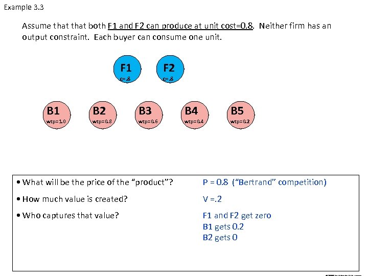
Example 3. 3 Assume that both F 1 and F 2 can produce at unit cost=0. 8. Neither firm has an output constraint. Each buyer can consume one unit. F 1 F 2 c=. 8 B 1 wtp=1. 0 B 2 wtp=0. 8 c=. 8 B 3 wtp=0. 6 B 4 wtp=0. 4 B 5 wtp=0. 2 • What will be the price of the “product”? P = 0. 8 (“Bertrand” competition) • How much value is created? V =. 2 • Who captures that value? F 1 and F 2 get zero B 1 gets 0. 2 B 2 gets 0

Example 3. 4 Now assume that F 1 has a “cost advantage” and can produce at cost 0, but F 2 has unit cost=0. 8. Neither firm has an output constraint. F 1 F 2 c=0 B 1 wtp=1. 0 B 2 wtp=0. 8 c=. 8 B 3 wtp=0. 6 B 4 wtp=0. 4 B 5 wtp=0. 2 In this case F 1 has a big cost advantage and can drive F 2 out of the market. F 1 maximizes profit by charging a price of $. 60, just like the monopolist in Example 1. 5 from Lecture 1. • What will be the price of the “product”? P = 0. 6 • How much value is created? V = 2. 4 (= 1 +. 8 +. 6) • Who captures that value? F 1 gets 1. 8; F 2 gets zero B 1 gets 0. 4 B 2 gets 0. 2 B 3 gets 0 So, F 1’s cost advantage creates additional value of 2. 2 (= 2. 4 – 0. 2), which is split between F 1 and its
Now, let’s increase the number of firms and consider how the heterogeneity of sellers and buyers leads to the economic concept of supply and demand curves.
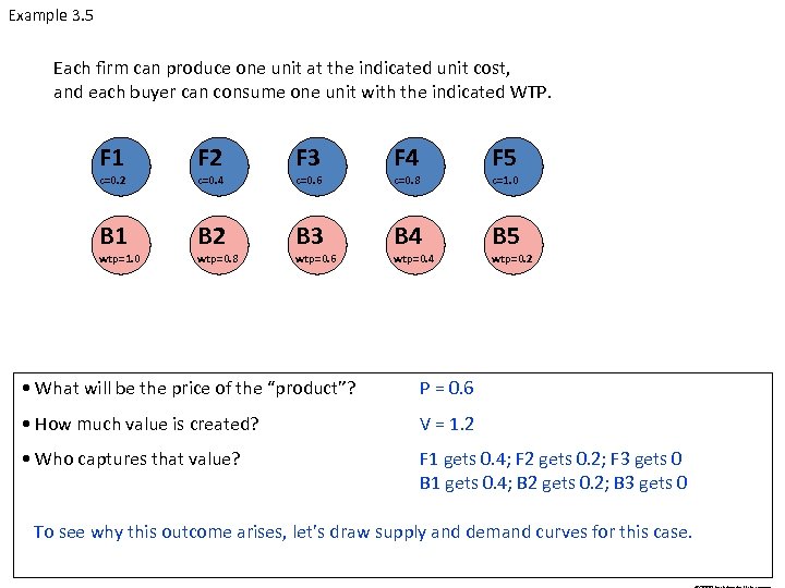
Example 3. 5 Each firm can produce one unit at the indicated unit cost, and each buyer can consume one unit with the indicated WTP. F 1 F 2 F 3 F 4 F 5 B 1 B 2 B 3 B 4 B 5 c=0. 2 wtp=1. 0 c=0. 4 wtp=0. 8 c=0. 6 wtp=0. 6 c=0. 8 wtp=0. 4 c=1. 0 wtp=0. 2 • What will be the price of the “product”? P = 0. 6 • How much value is created? V = 1. 2 • Who captures that value? F 1 gets 0. 4; F 2 gets 0. 2; F 3 gets 0 B 1 gets 0. 4; B 2 gets 0. 2; B 3 gets 0 To see why this outcome arises, let’s draw supply and demand curves for this case.
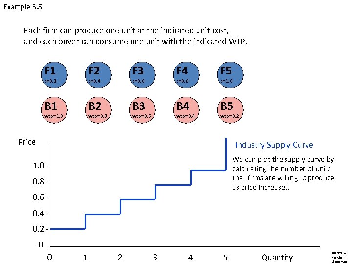
Example 3. 5 Each firm can produce one unit at the indicated unit cost, and each buyer can consume one unit with the indicated WTP. F 1 F 2 F 3 F 4 F 5 B 1 B 2 B 3 B 4 B 5 c=0. 2 c=0. 4 wtp=1. 0 c=0. 6 wtp=0. 8 c=0. 8 wtp=0. 6 wtp=0. 4 c=1. 0 wtp=0. 2 Price Industry Supply Curve We can plot the supply curve by calculating the number of units that firms are willing to produce as price increases. 1. 0 0. 8 0. 6 0. 4 0. 2 0 0 1 2 3 4 5 Quantity © 2009 by Marvin Lieberman
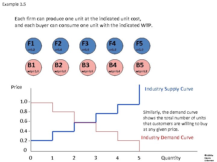
Example 3. 5 Each firm can produce one unit at the indicated unit cost, and each buyer can consume one unit with the indicated WTP. F 1 F 2 F 3 F 4 F 5 B 1 B 2 B 3 B 4 B 5 c=0. 2 c=0. 4 wtp=1. 0 c=0. 6 wtp=0. 8 c=0. 8 wtp=0. 6 wtp=0. 4 c=1. 0 wtp=0. 2 Price Industry Supply Curve 1. 0 0. 8 - Similarly, the demand curve shows the total number of units that customers are willing to buy at any given price. 0. 6 0. 4 - Industry Demand Curve 0. 2 0 0 1 2 3 4 5 Quantity © 2009 by Marvin Lieberman

Example 3. 5 Each firm can produce one unit at the indicated unit cost, and each buyer can consume one unit with the indicated WTP. F 1 F 2 F 3 F 4 F 5 B 1 B 2 B 3 B 4 B 5 c=0. 2 c=0. 4 wtp=1. 0 c=0. 6 wtp=0. 8 c=0. 8 wtp=0. 6 wtp=0. 4 c=1. 0 wtp=0. 2 This area corresponds to industry profit, called “producer surplus” in economics. It is the economic value that is captured by producers (F 1 and F 2 in this example). Price 1. 0 0. 8 - Industry Supply Curve 0. 6 0. 4 Industry Demand Curve 0. 2 0 0 1 2 3 4 5 Quantity © 2009 by Marvin Lieberman
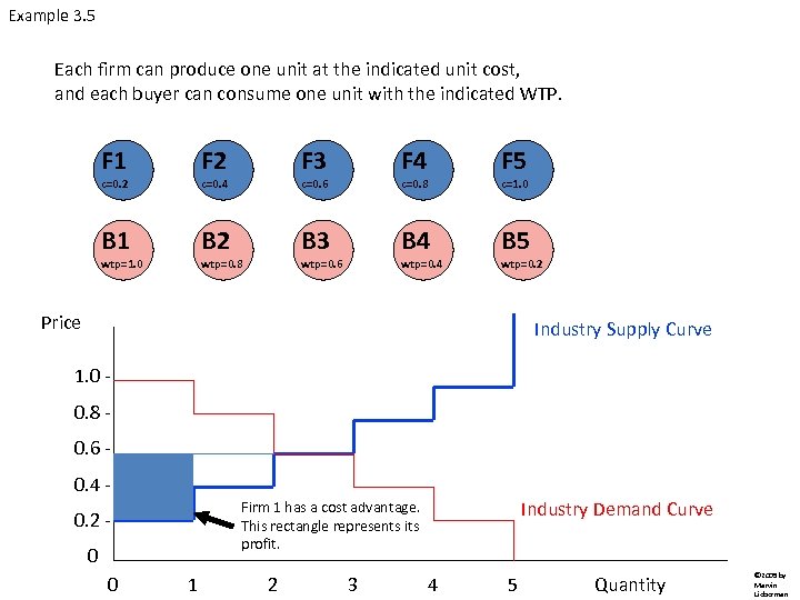
Example 3. 5 Each firm can produce one unit at the indicated unit cost, and each buyer can consume one unit with the indicated WTP. F 1 F 2 F 3 F 4 F 5 B 1 B 2 B 3 B 4 B 5 c=0. 2 c=0. 4 wtp=1. 0 c=0. 6 wtp=0. 8 c=0. 8 wtp=0. 6 wtp=0. 4 c=1. 0 wtp=0. 2 Price Industry Supply Curve 1. 0 0. 8 0. 6 0. 4 0 0 Industry Demand Curve Firm 1 has a cost advantage. This rectangle represents its profit. 0. 2 1 2 3 4 5 Quantity © 2009 by Marvin Lieberman

Example 3. 5 Each firm can produce one unit at the indicated unit cost, and each buyer can consume one unit with the indicated WTP. F 1 F 2 F 3 F 4 F 5 B 1 B 2 B 3 B 4 B 5 c=0. 2 c=0. 4 wtp=1. 0 c=0. 6 wtp=0. 8 c=0. 8 wtp=0. 6 wtp=0. 4 c=1. 0 wtp=0. 2 Price Industry Supply Curve 1. 0 0. 8 0. 6 0. 4 0 0 Industry Demand Curve Firm 2 also has a cost advantage, albeit smaller than F 1’s. This rectangle represents F 2’s profit. 0. 2 1 2 3 4 5 Quantity © 2009 by Marvin Lieberman
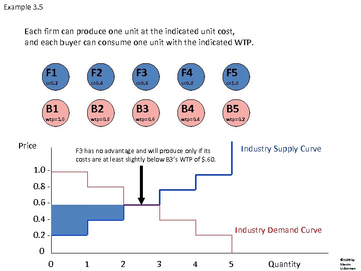
Example 3. 5 Each firm can produce one unit at the indicated unit cost, and each buyer can consume one unit with the indicated WTP. F 1 F 2 F 3 F 4 F 5 B 1 B 2 B 3 B 4 B 5 c=0. 2 c=0. 4 wtp=1. 0 Price c=0. 6 wtp=0. 8 c=0. 8 wtp=0. 6 wtp=0. 4 c=1. 0 wtp=0. 2 Industry Supply Curve F 3 has no advantage and will produce only if its costs are at least slightly below B 3’s WTP of $. 60. 1. 0 0. 8 0. 6 0. 4 Industry Demand Curve 0. 2 0 0 1 2 3 4 5 Quantity © 2009 by Marvin Lieberman

Example 3. 5 Each firm can produce one unit at the indicated unit cost, and each buyer can consume one unit with the indicated WTP. F 1 F 2 F 3 F 4 F 5 B 1 B 2 B 3 B 4 B 5 c=0. 2 c=0. 4 wtp=1. 0 c=0. 6 wtp=0. 8 c=0. 8 wtp=0. 6 wtp=0. 4 c=1. 0 wtp=0. 2 Price Industry Supply Curve The supply and demand curves have a stair step shape in these examples, given the small number of buyers and sellers. The curves become smoother when the number of firms and customers increases. 1. 0 0. 8 0. 6 0. 4 - Industry Demand Curve 0. 2 0 0 1 2 3 4 5 Quantity © 2009 by Marvin Lieberman

Now, let’s consider some cases with “differentiation advantage. ” Differentiation advantage is a bit more complicated than cost advantage, as it is necessary to introduce the notion of product quality. Differentiation advantage can arise if the buyers’ WTP differs among products offered by the competing firms. We will consider examples with two firms facing two buyers. For comparison purposes, let’s start with a base case where there is no difference between the firms or their products. © 2009 by Marvin Lieberman

Example 3. 6 Two firms, each able to produce “product” at cost=0 with no capacity constraints. F 1 c=0 B 1 wtp=1 F 2 c=0 B 2 wtp=1 Two buyers, each able to consume one unit of the “product” and willing to pay at most $1. (i. e. , the value to each buyer of consuming the product is $1. ) In the absence of differentiation, price falls to zero (or just slightly above) and neither firm makes any profit. It is hard to make money in a commodity product industry unless there are capacity constraints or differential costs – or collusion among producers. • What will be the price of the “product”? P = 0 (“Bertrand competition”) • How much value is created? V = 2 • Who captures that value? B 1 and B 2 each get $1. F 1 and F 2 make no profit. © 2009 by Marvin Lieberman
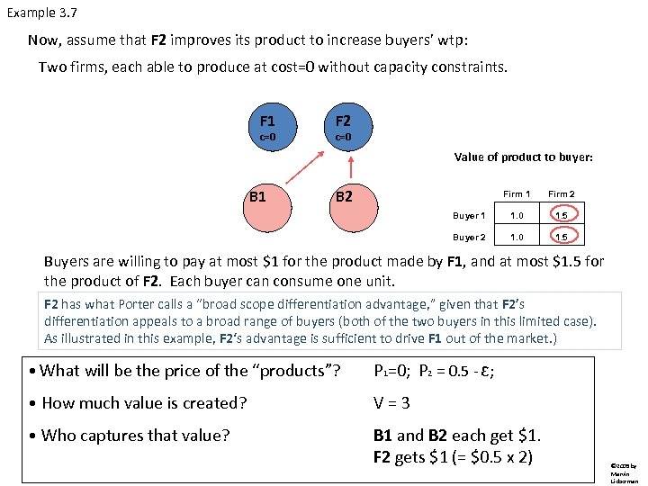
Example 3. 7 Now, assume that F 2 improves its product to increase buyers’ wtp: Two firms, each able to produce at cost=0 without capacity constraints. F 1 c=0 F 2 c=0 Value of product to buyer: B 1 B 2 Firm 1 Firm 2 Buyer 1 1. 0 1. 5 Buyer 2 1. 0 1. 5 Buyers are willing to pay at most $1 for the product made by F 1, and at most $1. 5 for the product of F 2. Each buyer can consume one unit. F 2 has what Porter calls a “broad scope differentiation advantage, ” given that F 2’s differentiation appeals to a broad range of buyers (both of the two buyers in this limited case). As illustrated in this example, F 2‘s advantage is sufficient to drive F 1 out of the market. ) • What will be the price of the “products”? P 1=0; P 2 = 0. 5 - ε; • How much value is created? V = 3 • Who captures that value? B 1 and B 2 each get $1. F 2 gets $1 (= $0. 5 x 2) © 2009 by Marvin Lieberman
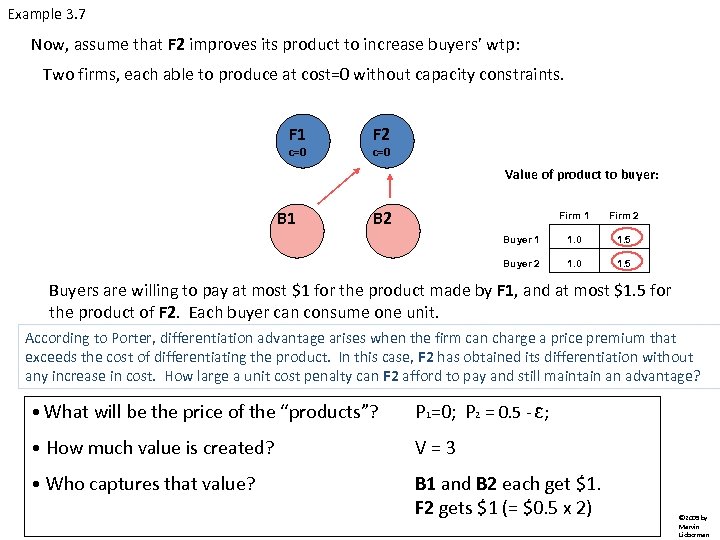
Example 3. 7 Now, assume that F 2 improves its product to increase buyers’ wtp: Two firms, each able to produce at cost=0 without capacity constraints. F 1 c=0 F 2 c=0 Value of product to buyer: B 1 B 2 Firm 1 Firm 2 Buyer 1 1. 0 1. 5 Buyer 2 1. 0 1. 5 Buyers are willing to pay at most $1 for the product made by F 1, and at most $1. 5 for the product of F 2. Each buyer can consume one unit. According to Porter, differentiation advantage arises when the firm can charge a price premium that exceeds the cost of differentiating the product. In this case, F 2 has obtained its differentiation without any increase in cost. How large a unit cost penalty can F 2 afford to pay and still maintain an advantage? • What will be the price of the “products”? P 1=0; P 2 = 0. 5 - ε; • How much value is created? V = 3 • Who captures that value? B 1 and B 2 each get $1. F 2 gets $1 (= $0. 5 x 2) © 2009 by Marvin Lieberman

Example 3. 7 Now, assume that F 2 improves its product to increase buyers’ wtp: Two firms, each able to produce at cost=0 without capacity constraints. F 1 c=0 F 2 c=0 Value of product to buyer: B 1 B 2 Firm 1 Firm 2 Buyer 1 1. 0 1. 5 Buyer 2 1. 0 1. 5 Buyers are willing to pay at most $1 for the product made by F 1, and at most $1. 5 for the product of F 2. Each buyer can consume one unit. Answer: F 2 maintains an advantage as long as its cost remain below $. 50. So, if F 2 incurred costs of $. 40 per unit to achieve its differentiation, it would still have a competitive advantage. • What will be the price of the “products”? P 1=0; P 2 = 0. 5 - ε; • How much value is created? V = 3 • Who captures that value? B 1 and B 2 each get $1. F 2 gets $1 (= $0. 5 x 2) © 2009 by Marvin Lieberman

In the previous example, Firm 2’s advantage comes from what economists call vertical product differentiation. Differentiation of this type makes the firm’s product more attractive to all potential customers. In the example, both buyers consider the differentiated product to be of higher quality and are willing to pay more for it. (The term vertical comes from the fact that all customers have the same ordering of product quality from high to low. ) Another type of differentiation is what economists call horizontal product differentiation. With horizontal differentiation, buyers differ in their tastes and preferences. Let’s see what happens when the market offers opportunities for horizontal product differentiation. © 2009 by Marvin Lieberman
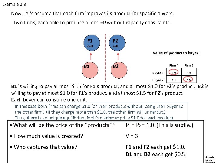
Example 3. 8 Now, let’s assume that each firm improves its product for specific buyers: Two firms, each able to produce at cost=0 without capacity constraints. F 1 c=0 F 2 c=0 Value of product to buyer: B 1 B 2 Firm 1 Firm 2 Buyer 1 1. 5 1. 0 Buyer 2 1. 0 1. 5 B 1 is willing to pay at most $1. 5 for F 1’s product, and at most $1. 0 for F 2’s product. B 2 is willing to pay at most $1. 0 for F 1’s product, and at most $1. 5 for F 2’s product. Each buyer can consume one unit. In this case both firms can charge $1. 0 for their products without losing their buyer to the other firm. (If they charge more than $1. 0, the other firm will undercut. ) Thus, there is an unique equilibrium in this market at price $1. 0 for each product. • What will be the price of the “products”? P 1 = P 2 = 1. 0 (This is subtle. ) • How much value is created? V = 3 • Who captures that value? F 1 and F 2 each get $1. 0. B 1 and B 2 each get $0. 5. © 2009 by Marvin Lieberman

Example 3. 8 Now, let’s assume that each firm improves its product for specific buyers: Two firms, each able to produce at cost=0 without capacity constraints. F 1 c=0 F 2 c=0 Value of product to buyer: B 1 B 2 Firm 1 Firm 2 Buyer 1 1. 5 1. 0 Buyer 2 1. 0 1. 5 B 1 is willing to pay at most $1. 5 for F 1’s product, and at most $1. 0 for F 2’s product. B 2 is willing to pay at most $1. 0 for F 1’s product, and at most $1. 5 for F 2’s product. Each buyer can consume one unit. Note that each firm captures a different buyer “segment. ” The firms enjoy an added benefit in that “rivalry” is diminished. • What will be the price of the “products”? P 1 = P 2 = 1. 0 (This is subtle. ) • How much value is created? V = 3 • Who captures that value? F 1 and F 2 each get $1. 0. B 1 and B 2 each get $0. 5. © 2009 by Marvin Lieberman
This case illustrates a number of features about differentiation advantage: Ø By appealing to different market “segments, ” many firms can enjoy differentiation advantage within the same industry. Both firms in Example 3. 8 have a differentiation advantage, and they earn identical profits. Thus, differentiation advantage need not be earned by one firm at the expense of another. This differs from cost advantage, where profits are determined by a given firm’s cost position relative to other firms in the market. Ø Although not addressed in the previous lecture on how Porter's Five Forces influence the distribution of profits in an industry, product differentiation tends to diminish the rivalry among firms. As a result, industries with high product differentiation often have a relatively large number of firms with high profitability. We see this in Example 3. 8, where the fact that the firms are pursuing different customers reduces the intensity of price competition. © 2009 by Marvin Lieberman

A closing footnote on defining “competitive advantage”: As noted at the start of this lecture, there is currently debate the field of business strategy about the appropriate definition of "competitive advantage". In our last example, both firms earned attractive returns by differentiating their products. Their profits were equal, and neither firm was superior to the other. We have described this as a case where both firms have achieved competitive advantage. But those who define advantage as superiority over rivals within a specific market would argue that neither firm has a competitive advantage in this case. (At issue is whether the profits from differentiation should be attributed to the industry or to the firm. ) In our previous examples where one firm has lower cost than rivals, "competitive advantage" may depend on how the value created by the firm is distributed among stakeholders. If this value flows to shareholders in the form of profits, few would question that the firm has competitive advantage. However, if this value is captured by the firm's management and employees, many would argue that the firm lacks competitive advantage, even though the firm may be far more efficient than its rivals. For instance, consider an industry where one firm, through the cooperation of management and labor, is able to produce a given output with only half the number of employees as competitors. If the resulting surplus is paid out to shareholders, there is little question that the firm enjoys a competitive advantage. However, if the surplus is captured entirely by managers and workers in the form of higher salaries, wages or bonuses, many would argue that the firm does not have competitive advantage. (The claim in this case is that the firm has an advantage in "efficiency" but not in "cost". ) Thus, the existence and magnitude of "competitive advantage“ depends on how the concept is defined. © 2009 by Marvin Lieberman
This concludes our analysis of cost and differentiation advantage. The most basic points to remember are the following: § Cost advantage arises when firms are heterogeneous in their cost positions. § Differentiation advantage arises when a firm is able to enhance the quality of its product(s) in a way that raises buyer's WTP (and hence the price charged by the firm) by more than the cost of achieving differentiation. While we have established some conceptual foundations for understanding these two forms of competitive advantage, we have said nothing about how firms are able to achieve low cost or high quality positions in practice. Those managerial challenges are fundamental, but they lie beyond the scope of these brief lectures. Many of the tactics for gaining competitive advantage are addressed in strategic management, marketing and operations courses. Hopefully, these lectures have prepared you to think about those courses, and about business in general, in terms of value creation and capture. © 2009 by Marvin Lieberman
8b425c6ffd92a3075a321596ddcc5622.ppt