Introduction to Business Management: Statistics Class 3 Topic

Introduction to Business Management: Statistics Class 3 Topic 4. Descriptive statistics Measures of central tendency Variation and shape

In this topic you learn To describe the properties of central tendency, variation, and shape in numerical data To calculate descriptive summary measures for a population To construct and interpret a boxplot
Planned 4.1 Measures of central tendency and characteristics of the distribution center. 4.2 Measures of variation and the shape of the distribution. Z-scores. 4.3 Characteristics of the population: parameters. 4.4 The empirical rule and the Chebyshev Rule. 4.5 Characteristics of samples: parameters estimation.

Live Exercise Ethan and Cindy decide to buy a car. They’ve visited 7 markets and tested 7 cars Toyota and KIA (the same model). They put 10 liters of gasoline and drive on a closed track until it runs out gas. The results are: Which model is better? Please, take your calculators and help!
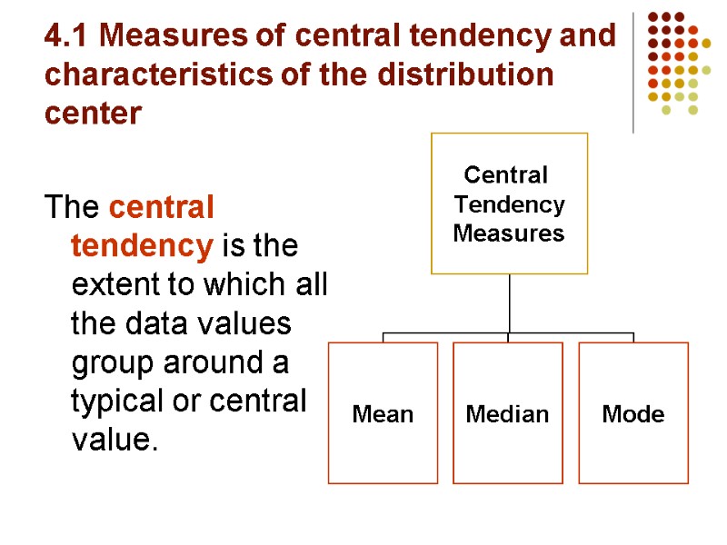
4.1 Measures of central tendency and characteristics of the distribution center The central tendency is the extent to which all the data values group around a typical or central value.
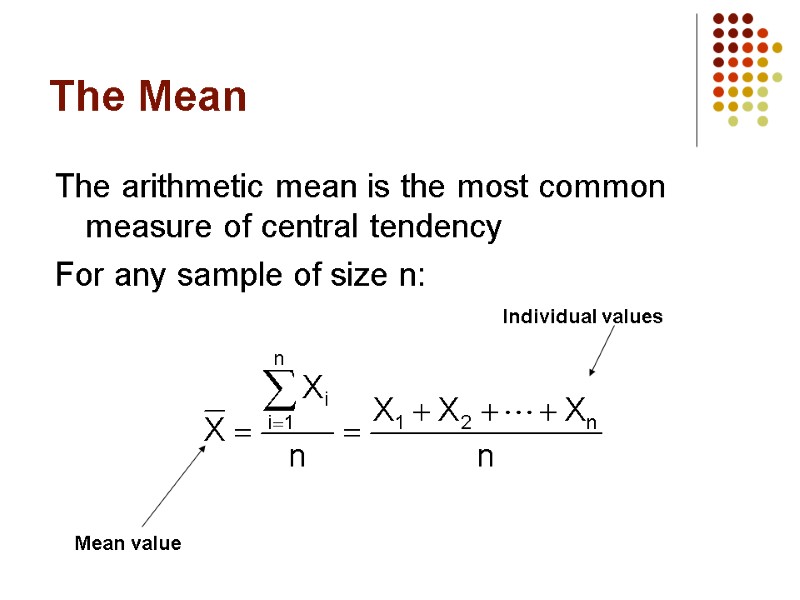
The Mean The arithmetic mean is the most common measure of central tendency For any sample of size n:
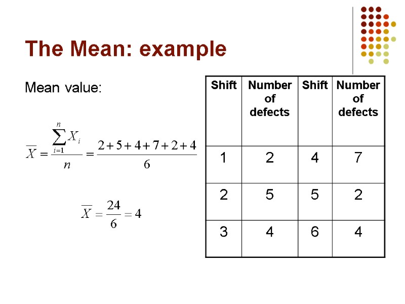
The Mean: example Mean value:
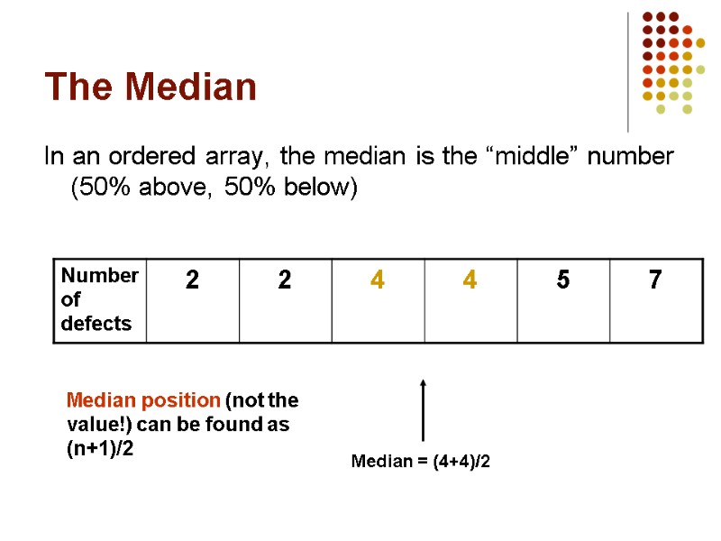
The Median In an ordered array, the median is the “middle” number (50% above, 50% below) Median position (not the value!) can be found as (n+1)/2
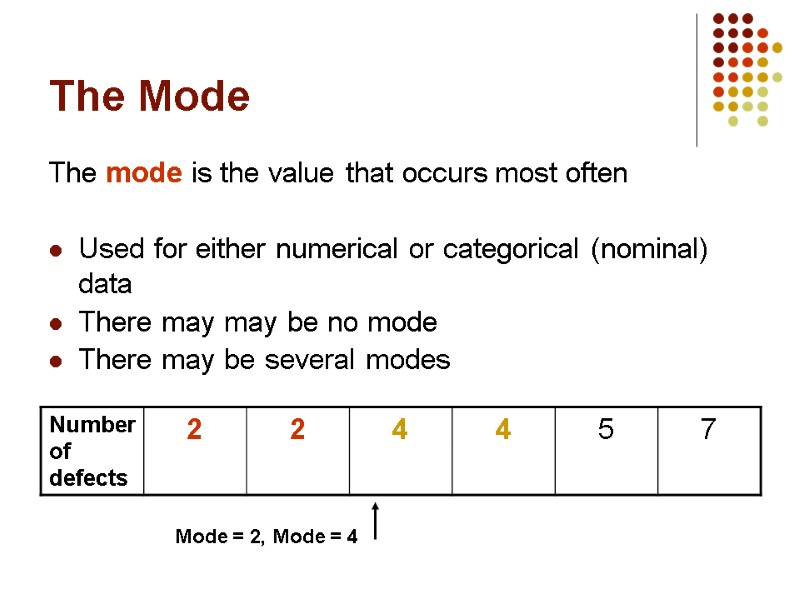
The Mode The mode is the value that occurs most often Used for either numerical or categorical (nominal) data There may may be no mode There may be several modes

Which Measure to Choose? The mean is generally used, unless extreme values (outliers) exist. The median is often used, since the median is not sensitive to extreme values. For example, median home prices may be reported for a region; it is less sensitive to outliers. In some situations it makes sense to report both the mean and the median. Mean, …
Shape of a distribution and central tendency measures The shape is the pattern of the distribution of values from the lowest value to the highest value.
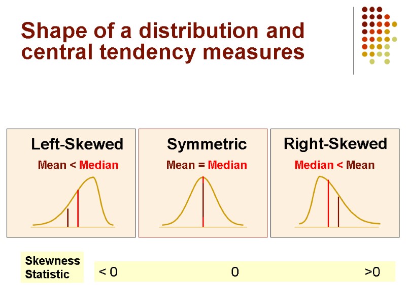
Shape of a distribution and central tendency measures Mean = Median Mean < Median Median < Mean Right-Skewed Left-Skewed Symmetric Skewness Statistic < 0 0 >0
Planned 4.1 Measures of central tendency and characteristics of the distribution center. 4.2 Measures of variation and the shape of the distribution. Z-scores. 4.3 Characteristics of the population: parameters. 4.4 The empirical rule and the Chebyshev Rule. 4.5 Characteristics of samples: parameters estimation.
![Variation is… The term variability will be taken to mean the [varying] characteristic of Variation is… The term variability will be taken to mean the [varying] characteristic of](https://present5.com/presentacii-2/20171208\14082-topic_4.ppt\14082-topic_4_14.jpg)
Variation is… The term variability will be taken to mean the [varying] characteristic of the entity that is observable, and the term variation to mean the describing or measuring of that characteristic. Example: we’ll take 50 bottles of water (50ml) and measure the content. In each bottle we’ll found from 48 till 51 ml of water. Different in each bottle. It’s variability of the characteristics (content). We can describe it using mean value and individual differences (variation).
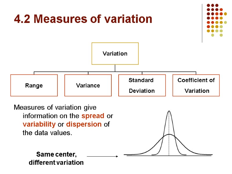
4.2 Measures of variation Measures of variation give information on the spread or variability or dispersion of the data values.
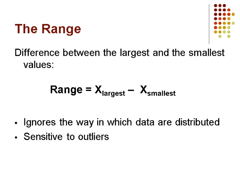
The Range Difference between the largest and the smallest values: Ignores the way in which data are distributed Sensitive to outliers Range = Xlargest – Xsmallest
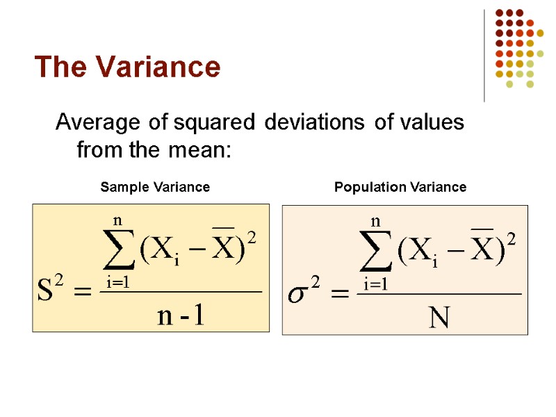
The Variance Average of squared deviations of values from the mean: Sample Variance Population Variance

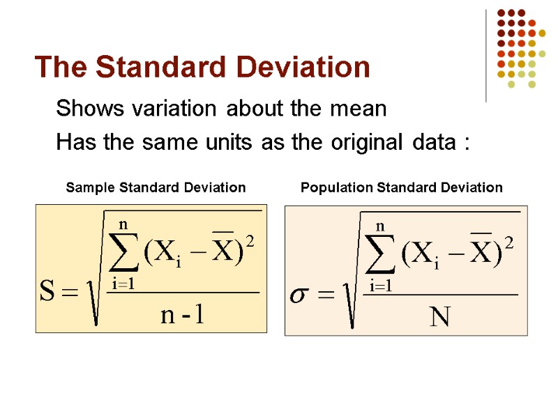
The Standard Deviation Shows variation about the mean Has the same units as the original data : Sample Standard Deviation Population Standard Deviation
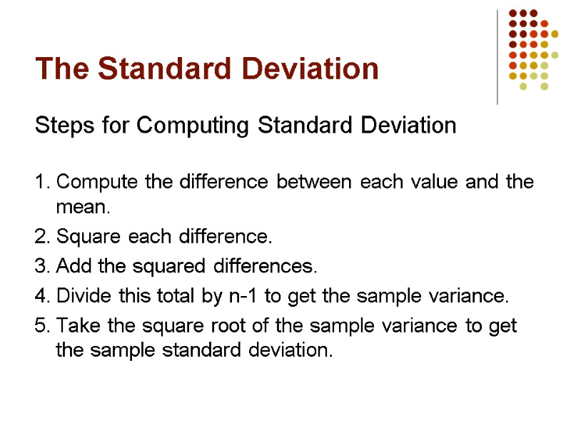
The Standard Deviation Steps for Computing Standard Deviation 1. Compute the difference between each value and the mean. 2. Square each difference. 3. Add the squared differences. 4. Divide this total by n-1 to get the sample variance. 5. Take the square root of the sample variance to get the sample standard deviation.
Measures of Variation: The more the data are spread out, the greater the range, variance, and standard deviation. The more the data are concentrated, the smaller the range, variance, and standard deviation. If the values are all the same (no variation), all these measures will be zero. None of these measures are ever negative.
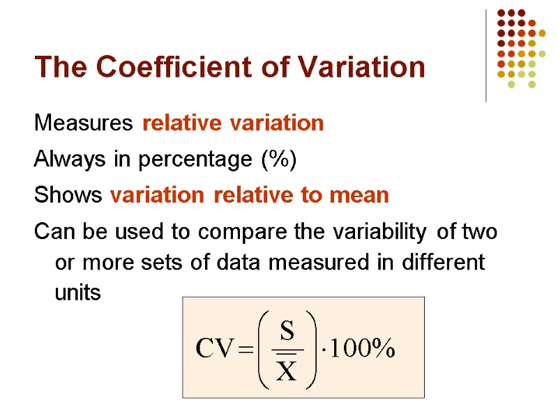
The Coefficient of Variation Measures relative variation Always in percentage (%) Shows variation relative to mean Can be used to compare the variability of two or more sets of data measured in different units
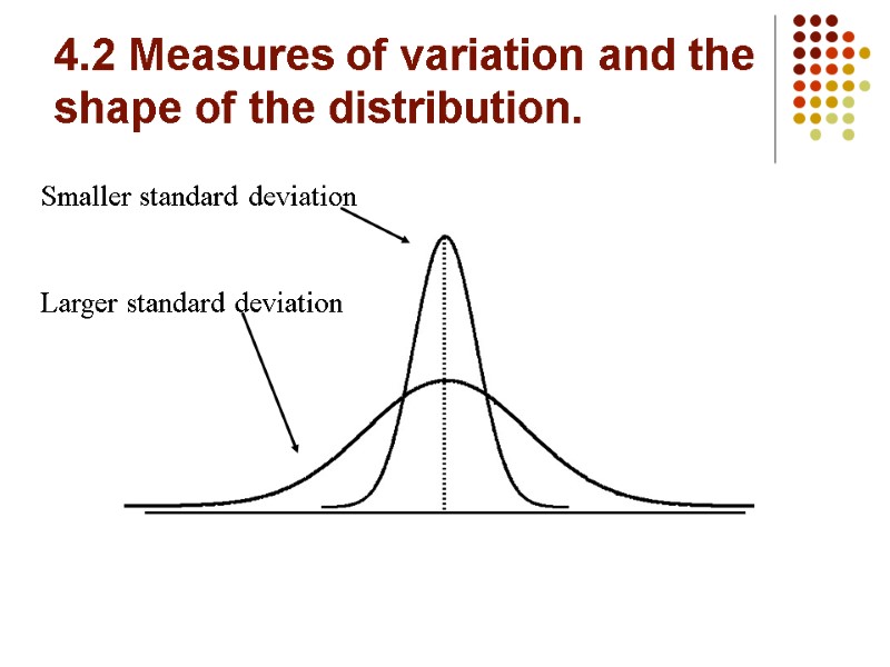
4.2 Measures of variation and the shape of the distribution. Smaller standard deviation Larger standard deviation
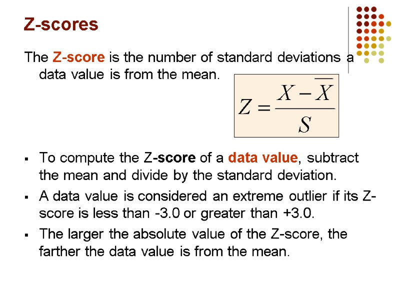
Z-scores The Z-score is the number of standard deviations a data value is from the mean. To compute the Z-score of a data value, subtract the mean and divide by the standard deviation. A data value is considered an extreme outlier if its Z-score is less than -3.0 or greater than +3.0. The larger the absolute value of the Z-score, the farther the data value is from the mean.
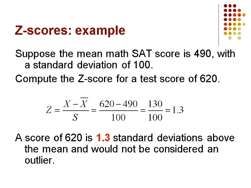
Z-scores: example Suppose the mean math SAT score is 490, with a standard deviation of 100. Compute the Z-score for a test score of 620. A score of 620 is 1.3 standard deviations above the mean and would not be considered an outlier.
Shape of a Distribution Describes how data are distributed Two useful shape related statistics are: Skewness Measures the amount of asymmetry in a distribution Kurtosis Measures the relative concentration of values in the center of a distribution as compared with the tails
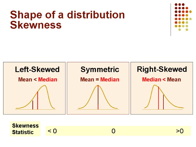
Shape of a distribution Skewness Mean = Median Mean < Median Median < Mean Right-Skewed Left-Skewed Symmetric Skewness Statistic < 0 0 >0
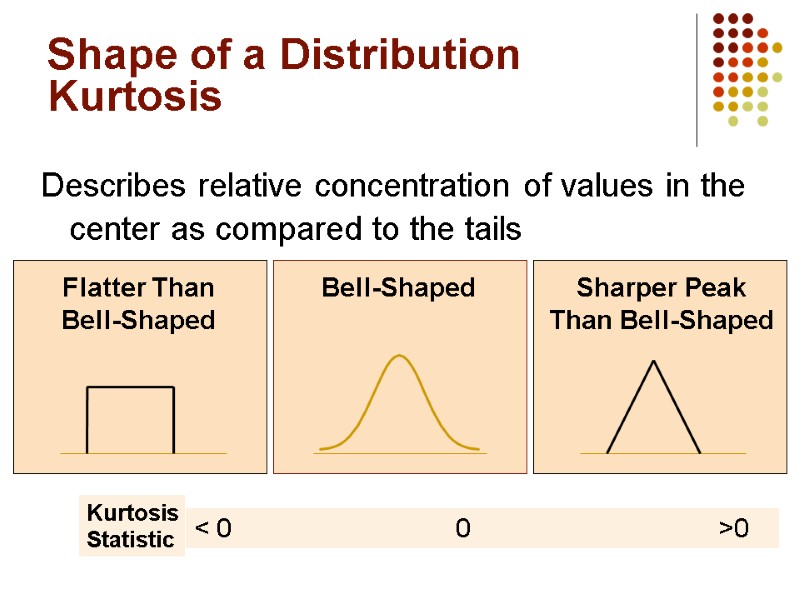
Shape of a Distribution Kurtosis Describes relative concentration of values in the center as compared to the tails Sharper Peak Than Bell-Shaped Flatter Than Bell-Shaped Bell-Shaped Kurtosis Statistic < 0 0 >0
The Five Number Summary The five numbers that help describe the center, spread and shape of data are: Xsmallest First Quartile (Q1) Median (Q2) Third Quartile (Q3) Xlargest
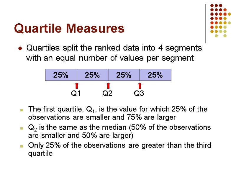
Quartile Measures Quartiles split the ranked data into 4 segments with an equal number of values per segment The first quartile, Q1, is the value for which 25% of the observations are smaller and 75% are larger Q2 is the same as the median (50% of the observations are smaller and 50% are larger) Only 25% of the observations are greater than the third quartile Q1 Q2 Q3
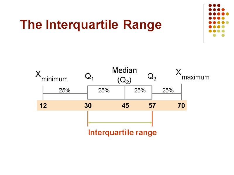
The Interquartile Range Median (Q2) X maximum X minimum Q1 Q3 25% 25% 25% 25% 12 30 45 57 70 Interquartile range
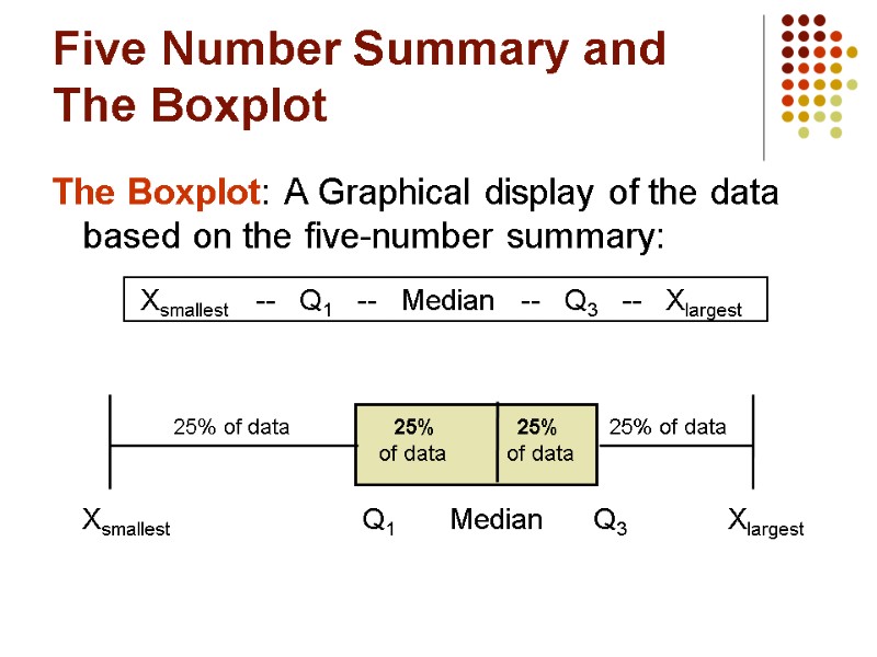
Five Number Summary and The Boxplot The Boxplot: A Graphical display of the data based on the five-number summary: Xsmallest -- Q1 -- Median -- Q3 -- Xlargest 25% of data 25% 25% 25% of data of data of data Xsmallest Q1 Median Q3 Xlargest
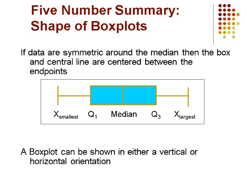
Five Number Summary: Shape of Boxplots If data are symmetric around the median then the box and central line are centered between the endpoints A Boxplot can be shown in either a vertical or horizontal orientation Xsmallest Q1 Median Q3 Xlargest
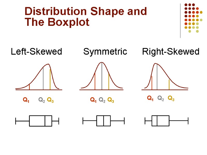
Distribution Shape and The Boxplot Right-Skewed Left-Skewed Symmetric Q1 Q2 Q3 Q1 Q2 Q3 Q1 Q2 Q3
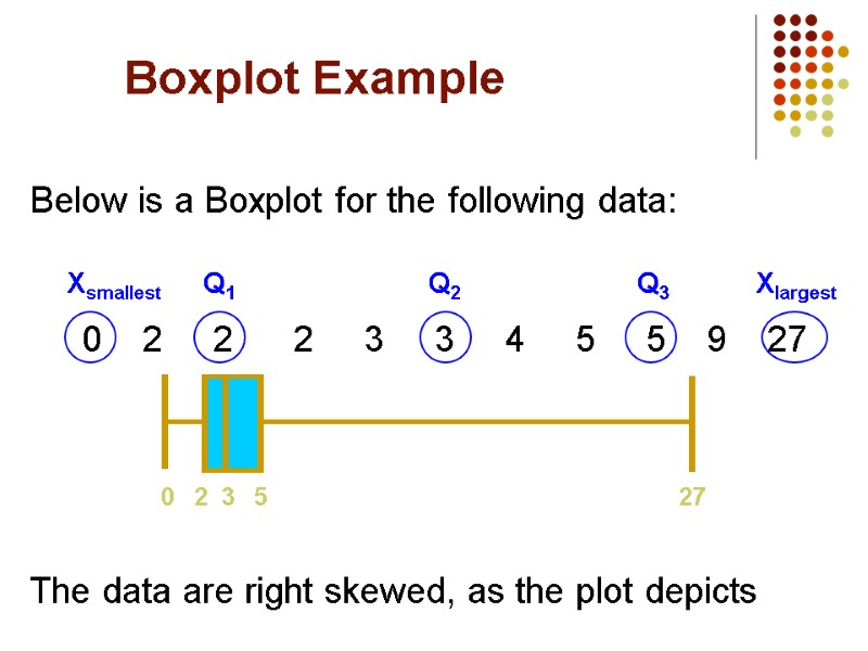
Boxplot Example Below is a Boxplot for the following data: 0 2 2 2 3 3 4 5 5 9 27 The data are right skewed, as the plot depicts 0 2 3 5 27 Xsmallest Q1 Q2 Q3 Xlargest
Planned 4.1 Measures of central tendency and characteristics of the distribution center. 4.2 Measures of variation and the shape of the distribution. Z-scores. 4.3 Characteristics of the population: parameters. 4.4 The empirical rule and the Chebyshev Rule. 4.5 Characteristics of samples: parameters estimation.
4.3 Characteristics of the population: parameters. Summary measures describing a population, called parameters, are denoted with Greek letters. Important population parameters are the population mean, variance, and standard deviation.

The Variance Average of squared deviations of values from the mean: Sample Variance Population Variance
The Standard Deviation Shows variation about the mean Has the same units as the original data : Sample Standard Deviation Population Standard Deviation
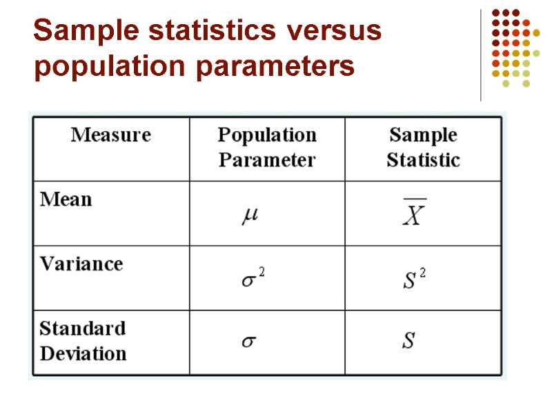
Sample statistics versus population parameters
Planned 4.1 Measures of central tendency and characteristics of the distribution center. 4.2 Measures of variation and the shape of the distribution. Z-scores. 4.3 Characteristics of the population: parameters. 4.4 The empirical rule and the Chebyshev Rule. 4.5 Characteristics of samples: parameters estimation.
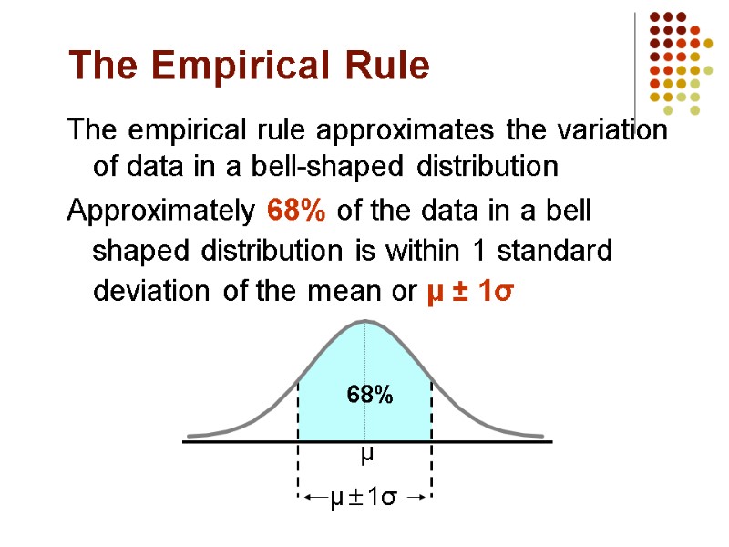
The empirical rule approximates the variation of data in a bell-shaped distribution Approximately 68% of the data in a bell shaped distribution is within 1 standard deviation of the mean or µ ± 1σ The Empirical Rule 68%
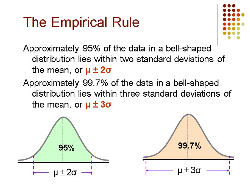
Approximately 95% of the data in a bell-shaped distribution lies within two standard deviations of the mean, or µ ± 2σ Approximately 99.7% of the data in a bell-shaped distribution lies within three standard deviations of the mean, or µ ± 3σ The Empirical Rule 99.7% 95%
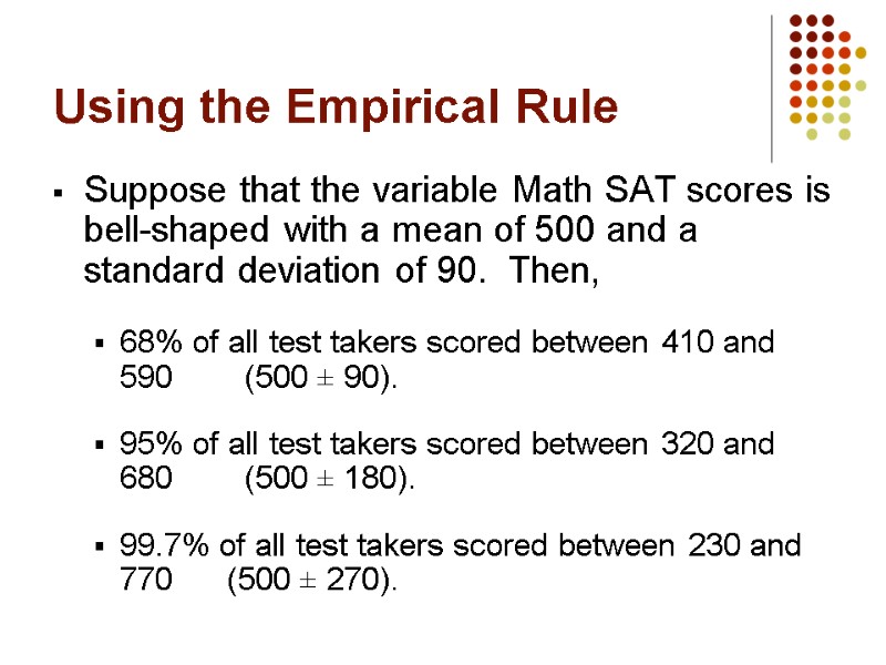
Using the Empirical Rule Suppose that the variable Math SAT scores is bell-shaped with a mean of 500 and a standard deviation of 90. Then, 68% of all test takers scored between 410 and 590 (500 ± 90). 95% of all test takers scored between 320 and 680 (500 ± 180). 99.7% of all test takers scored between 230 and 770 (500 ± 270).
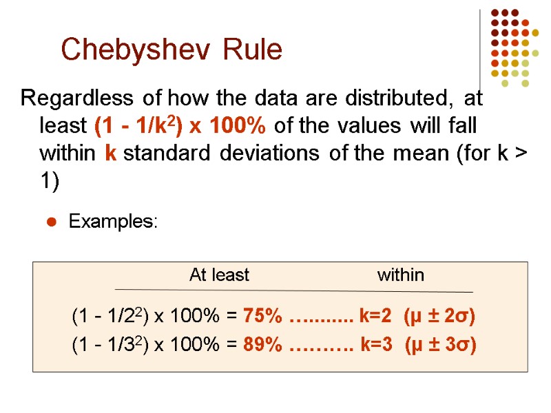
Regardless of how the data are distributed, at least (1 - 1/k2) x 100% of the values will fall within k standard deviations of the mean (for k > 1) Examples: (1 - 1/22) x 100% = 75% …........ k=2 (μ ± 2σ) (1 - 1/32) x 100% = 89% ………. k=3 (μ ± 3σ) Chebyshev Rule within At least
Planned 4.1 Measures of central tendency and characteristics of the distribution center. 4.2 Measures of variation and the shape of the distribution. Z-scores. 4.3 Characteristics of the population: parameters. 4.4 The empirical rule and the Chebyshev Rule. 4.5 Characteristics of samples: parameters estimation.
4.5 Characteristics of samples: parameters estimation The goal in sampling is to obtain individuals for a study in such a way that accurate information about the population can be obtained. Statistical inference is used for this purpose – special instrument, which allows to use information from a sample to draw conclusions about a population.
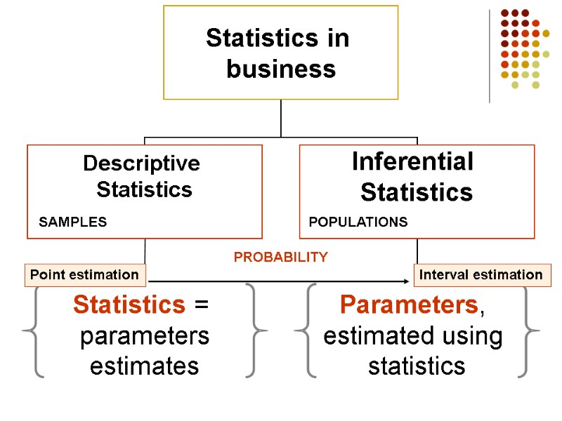
SAMPLES POPULATIONS

Assess your understanding Describe the relationship between variance and standard deviation. True of False? Chebyshev’s inequality applies to all distributions, but the Empirical Rule holds only for distributions that are bell-shaped. Describe how the mean and median can be used to determine the shape of the distribution.

In the Topic 4 we have Described measures of central tendency Mean, median, mode Described measures of variation Range, interquartile range, variance and standard deviation, coefficient of variation, Z-scores Illustrated shape of distribution Skewness & Kurtosis Described data using the 5-number summary Boxplots
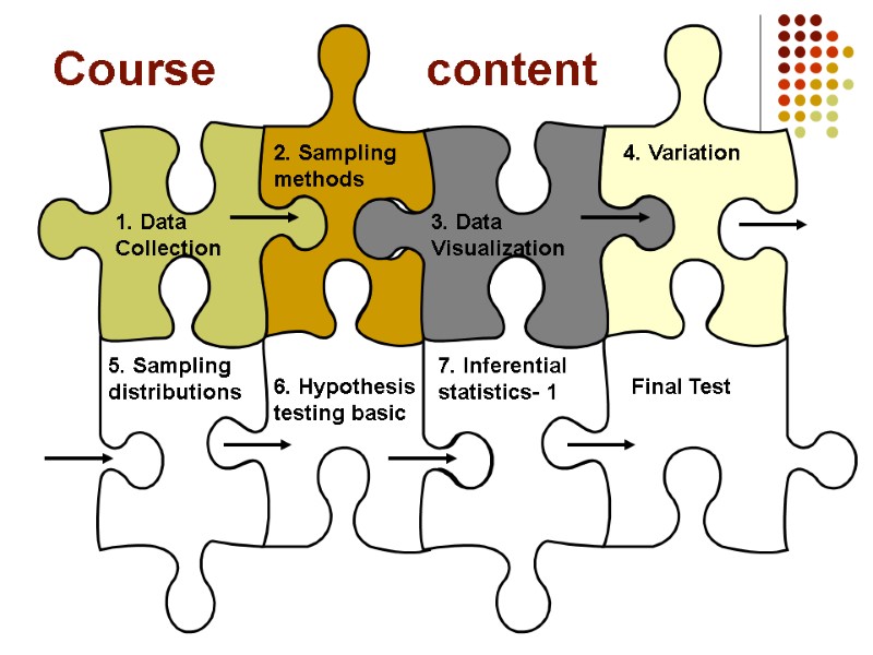
Course content 1. Data Collection 2. Sampling methods 3. Data Visualization 4. Variation 5. Sampling distributions 6. Hypothesis testing basic 7. Inferential statistics- 1 Final Test
Home Reading LSKB pages 112-159 Ex.3.50-3.61 (page 151) – to check your understanding Home assignment #2

Home assignment #2 Choose your favorite book (for example, Statistics for managers, by Levine at all…) Register prices for the book in 30 on-line shops, provide ordered array for prices and construct steam-and leaf plot. Compute the five-number summary. Draw a box plot of the data. Check the data set for outliers. Provide a short resume for your investigations (200-300 words, not more).
14082-topic_4.ppt
- Количество слайдов: 52

