INTRODUCTION TO ARTIFICIAL INTELLIGENCE Massimo Poesio LECTURE 15

INTRODUCTION TO ARTIFICIAL INTELLIGENCE Massimo Poesio LECTURE 15: Artificial Neural Networks

ARTIFICIAL NEURAL NETWORKS • Analogy to biological neural systems, the most robust learning systems we know. • Attempt to understand natural biological systems through computational modeling. • Massive parallelism allows for computational efficiency. • Help understand “distributed” nature of neural representations (rather than “localist” representation) that allow robustness and graceful degradation. • Intelligent behavior as an “emergent” property of large number of simple units rather than from explicitly encoded symbolic rules and algorithms. 2

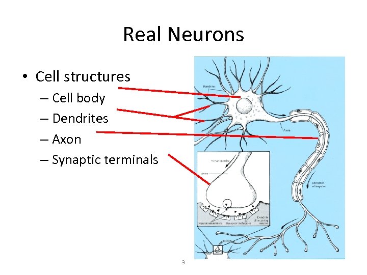Real Neurons • Cell structures – Cell body – Dendrites – Axon – Synaptic terminals 3

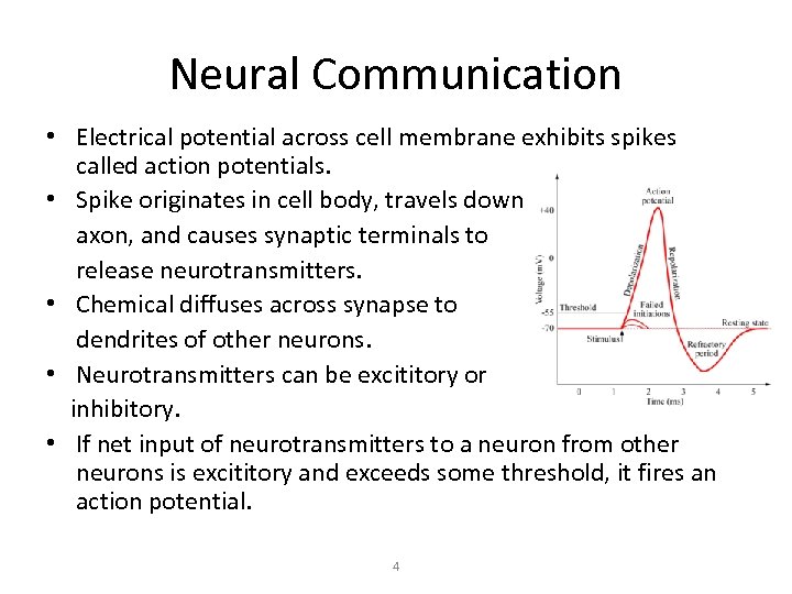Neural Communication • Electrical potential across cell membrane exhibits spikes called action potentials. • Spike originates in cell body, travels down axon, and causes synaptic terminals to release neurotransmitters. • Chemical diffuses across synapse to dendrites of other neurons. • Neurotransmitters can be excititory or inhibitory. • If net input of neurotransmitters to a neuron from other neurons is excititory and exceeds some threshold, it fires an action potential. 4

NEURAL SPEED CONSTRAINTS • Neurons have a “switching time” on the order of a few milliseconds, compared to nanoseconds for current computing hardware. • However, neural systems can perform complex cognitive tasks (vision, speech understanding) in tenths of a second. • Only time for performing 100 serial steps in this time frame, compared to orders of magnitude more for current computers. • Must be exploiting “massive parallelism. ” • Human brain has about 1011 neurons with an average of 104 connections each. 5

Real Neural Learning • Synapses change size and strength with experience. • Hebbian learning: When two connected neurons are firing at the same time, the strength of the synapse between them increases. • “Neurons that fire together, wire together. ” 6

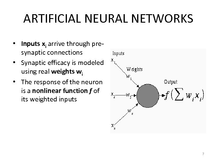ARTIFICIAL NEURAL NETWORKS • Inputs xi arrive through presynaptic connections • Synaptic efficacy is modeled using real weights wi • The response of the neuron is a nonlinear function f of its weighted inputs 7

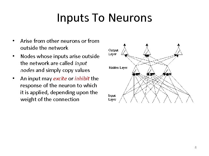Inputs To Neurons • Arise from other neurons or from outside the network • Nodes whose inputs arise outside the network are called input nodes and simply copy values • An input may excite or inhibit the response of the neuron to which it is applied, depending upon the weight of the connection 8

Weights • Represent synaptic efficacy and may be excitatory or inhibitory • Normally, positive weights are considered as excitatory while negative weights are thought of as inhibitory • Learning is the process of modifying the weights in order to produce a network that performs some function 9

ARTIFICIAL NEURAL NETWORK LEARNING • Learning approach based on modeling adaptation in biological neural systems. • Perceptron: Initial algorithm for learning simple neural networks (single layer) developed in the 1950’s. • Backpropagation: More complex algorithm for learning multi-layer neural networks developed in the 1980’s. 10

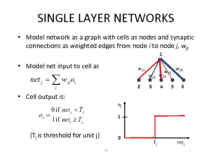SINGLE LAYER NETWORKS • Model network as a graph with cells as nodes and synaptic connections as weighted edges from node i to node j, wji 1 • Model net input to cell as w 12 2 w 15 w 13 w 14 3 4 5 w 16 6 • Cell output is: oj 1 (Tj is threshold for unit j) 0 11 Tj netj

Neural Computation • Mc. Collough and Pitts (1943) showed how single-layer neurons could compute logical functions and be used to construct finite-state machines. • Can be used to simulate logic gates: – AND: Let all wji be Tj/n, where n is the number of inputs. – OR: Let all wji be Tj – NOT: Let threshold be 0, single input with a negative weight. • Can build arbitrary logic circuits, sequential machines, and computers with such gates. • Given negated inputs, two layer network can compute any boolean function using a two level AND-OR network. 12

Perceptron Training • Assume supervised training examples giving the desired output for a unit given a set of known input activations. • Learn synaptic weights so that unit produces the correct output for each example. • Perceptron uses iterative update algorithm to learn a correct set of weights. 13

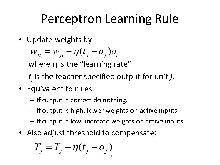Perceptron Learning Rule • Update weights by: where η is the “learning rate” tj is the teacher specified output for unit j. • Equivalent to rules: – If output is correct do nothing. – If output is high, lower weights on active inputs – If output is low, increase weights on active inputs • Also adjust threshold to compensate: 14

Perceptron Learning Algorithm • Iteratively update weights until convergence. Initialize weights to random values Until outputs of all training examples are correct For each training pair, E, do: Compute current output oj for E given its inputs Compare current output to target value, tj , for E Update synaptic weights and threshold using learning rule • Each execution of the outer loop is typically called an epoch. 15

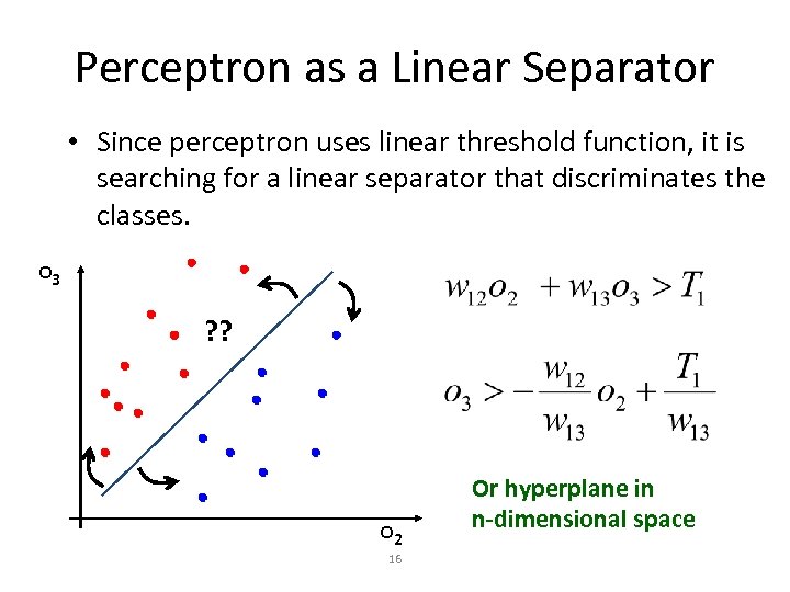Perceptron as a Linear Separator • Since perceptron uses linear threshold function, it is searching for a linear separator that discriminates the classes. o 3 ? ? o 2 16 Or hyperplane in n-dimensional space

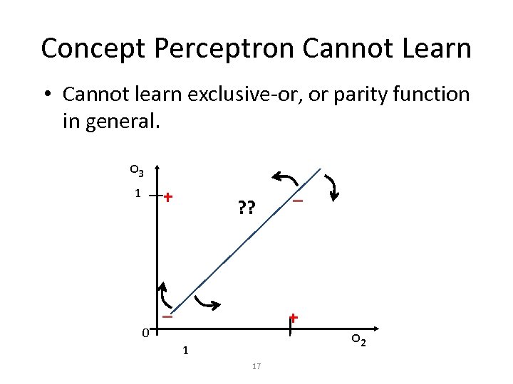Concept Perceptron Cannot Learn • Cannot learn exclusive-or, or parity function in general. o 3 + 1 0 ? ? – – + 1 17 o 2

Perceptron Limits • System obviously cannot learn concepts it cannot represent. • Minksy and Papert (1969) wrote a book analyzing the perceptron and demonstrating many functions it could not learn. • These results discouraged further research on neural nets; and symbolic AI became the dominate paradigm. 18

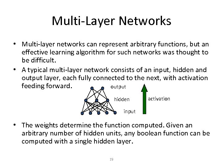Multi-Layer Networks • Multi-layer networks can represent arbitrary functions, but an effective learning algorithm for such networks was thought to be difficult. • A typical multi-layer network consists of an input, hidden and output layer, each fully connected to the next, with activation feeding forward. output hidden activation input • The weights determine the function computed. Given an arbitrary number of hidden units, any boolean function can be computed with a single hidden layer. 19

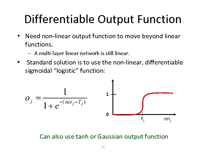Differentiable Output Function • Need non-linear output function to move beyond linear functions. – A multi-layer linear network is still linear. • Standard solution is to use the non-linear, differentiable sigmoidal “logistic” function: 1 0 Tj netj Can also use tanh or Gaussian output function 21

LEARNING WITH MULTI-LAYER NETWORKS • The BACKPROPAGATION algorithm allows to modify weights in a network consisting of several layers by ‘propagating back’ corrections

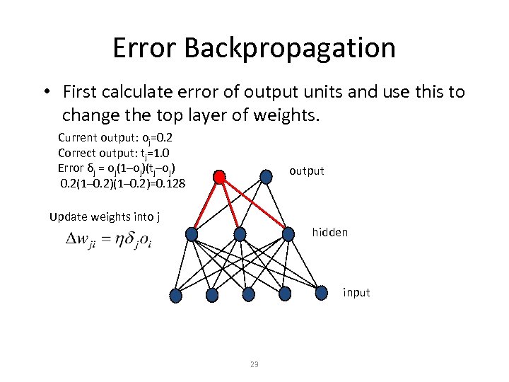Error Backpropagation • First calculate error of output units and use this to change the top layer of weights. Current output: oj=0. 2 Correct output: tj=1. 0 Error δj = oj(1–oj)(tj–oj) 0. 2(1– 0. 2)=0. 128 output Update weights into j hidden input 23

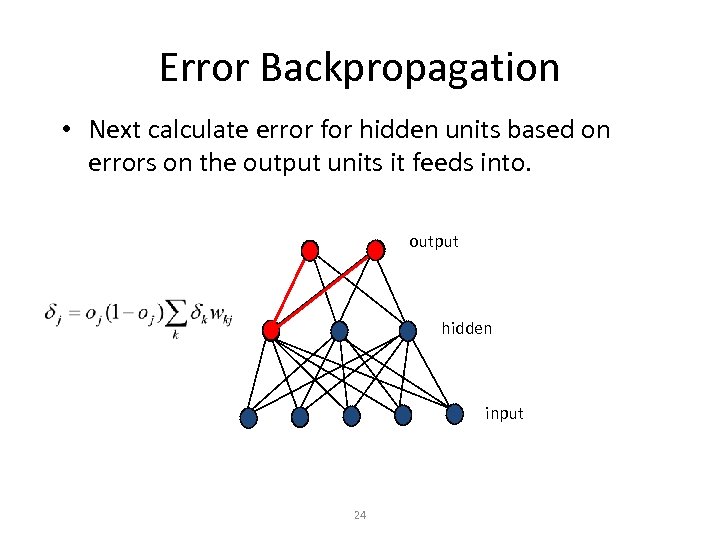Error Backpropagation • Next calculate error for hidden units based on errors on the output units it feeds into. output hidden input 24

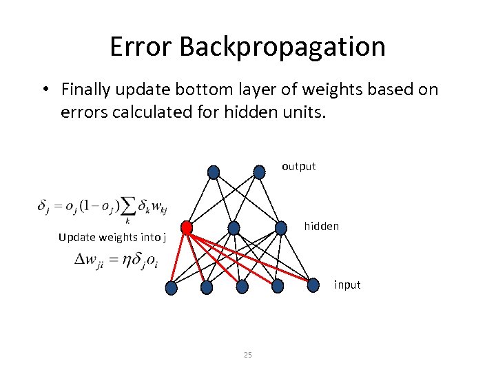Error Backpropagation • Finally update bottom layer of weights based on errors calculated for hidden units. output hidden Update weights into j input 25

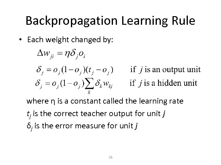Backpropagation Learning Rule • Each weight changed by: where η is a constant called the learning rate tj is the correct teacher output for unit j δj is the error measure for unit j 26

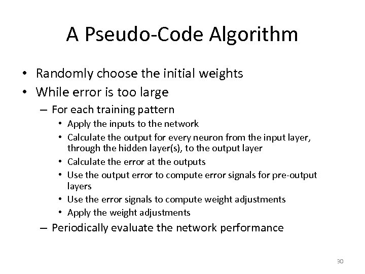A Pseudo-Code Algorithm • Randomly choose the initial weights • While error is too large – For each training pattern • Apply the inputs to the network • Calculate the output for every neuron from the input layer, through the hidden layer(s), to the output layer • Calculate the error at the outputs • Use the output error to compute error signals for pre-output layers • Use the error signals to compute weight adjustments • Apply the weight adjustments – Periodically evaluate the network performance 30

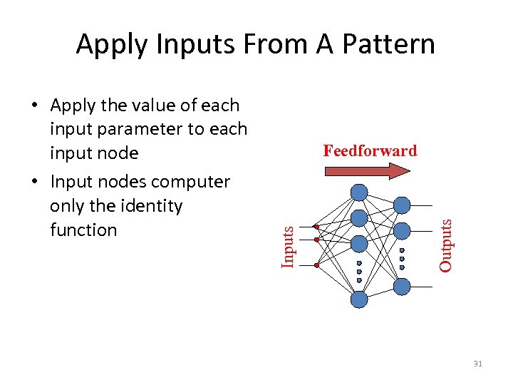Apply Inputs From A Pattern Outputs Feedforward Inputs • Apply the value of each input parameter to each input node • Input nodes computer only the identity function 31

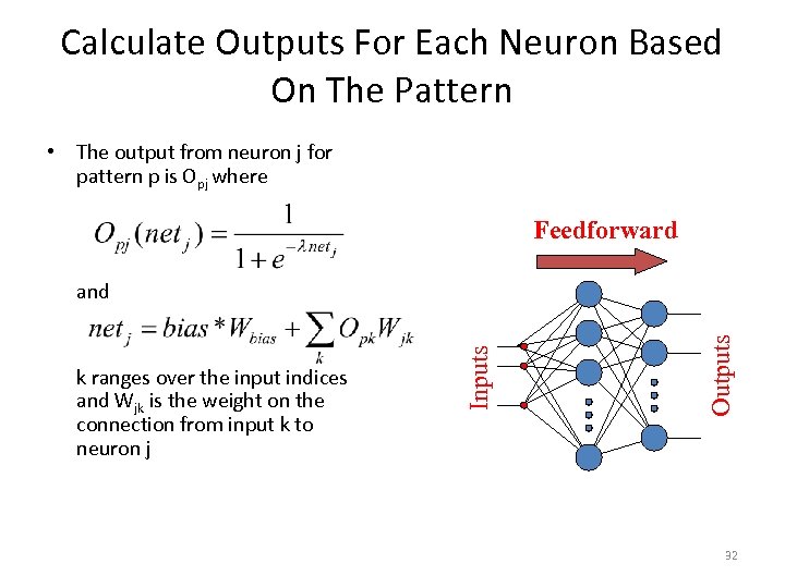Calculate Outputs For Each Neuron Based On The Pattern • The output from neuron j for pattern p is Opj where Feedforward Outputs k ranges over the input indices and Wjk is the weight on the connection from input k to neuron j Inputs and 32

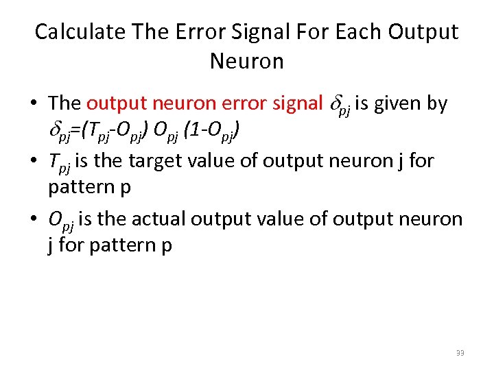Calculate The Error Signal For Each Output Neuron • The output neuron error signal dpj is given by dpj=(Tpj-Opj) Opj (1 -Opj) • Tpj is the target value of output neuron j for pattern p • Opj is the actual output value of output neuron j for pattern p 33

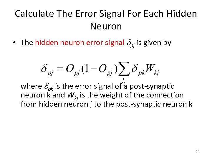Calculate The Error Signal For Each Hidden Neuron • The hidden neuron error signal dpj is given by where dpk is the error signal of a post-synaptic neuron k and Wkj is the weight of the connection from hidden neuron j to the post-synaptic neuron k 34

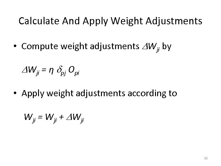Calculate And Apply Weight Adjustments • Compute weight adjustments DWji by DWji = η dpj Opi • Apply weight adjustments according to Wji = Wji + DWji 35

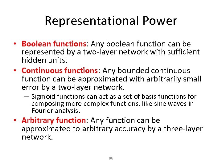Representational Power • Boolean functions: Any boolean function can be represented by a two-layer network with sufficient hidden units. • Continuous functions: Any bounded continuous function can be approximated with arbitrarily small error by a two-layer network. – Sigmoid functions can act as a set of basis functions for composing more complex functions, like sine waves in Fourier analysis. • Arbitrary function: Any function can be approximated to arbitrary accuracy by a three-layer network. 36

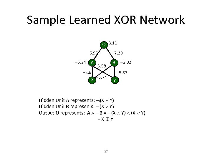Sample Learned XOR Network O 3. 11 7. 38 6. 96 5. 24 A 3. 6 X 3. 58 5. 74 B 2. 03 5. 57 Y Hidden Unit A represents: (X Y) Hidden Unit B represents: (X Y) Output O represents: A B = (X Y) =X Y 37

Hidden Unit Representations • Trained hidden units can be seen as newly constructed features that make the target concept linearly separable in the transformed space. • On many real domains, hidden units can be interpreted as representing meaningful features such as vowel detectors or edge detectors, etc. . • However, the hidden layer can also become a distributed representation of the input in which each individual unit is not easily interpretable as a meaningful feature. 38

Successful Applications • Text to Speech (Net. Talk) • Fraud detection • Financial Applications – HNC (eventually bought by Fair Isaac) • Chemical Plant Control – Pavillion Technologies • Automated Vehicles • Game Playing – Neurogammon • Handwriting recognition 39

Analysis of ANN Algorithm • Advantages: – Produce good results in complex domains – Suitable for both discrete and continuous data (especially better for the continuous domain) – Testing is very fast • Disadvantages: – Training is relatively slow – Learned results are difficult for users to interpret than learned rules (comparing with DT) – Empirical Risk Minimization (ERM) makes ANN try to minimize training error, may lead to overfitting 40

READINGS • Mitchell, Machine Learning, ch. 4

ACKNOWLEDGMENTS • Several slides come from Ray Mooney’s course on AI