Introduction So far we have optimization for a

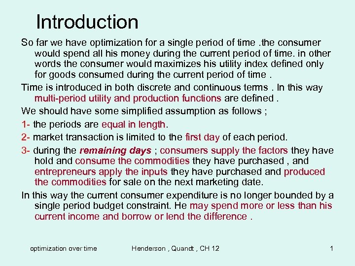Introduction So far we have optimization for a single period of time. the consumer would spend all his money during the current period of time. in other words the consumer would maximizes his utility index defined only for goods consumed during the current period of time. Time is introduced in both discrete and continuous terms. In this way multi-period utility and production functions are defined. We should have some simplified assumption as follows ; 1 - the periods are equal in length 2 - market transaction is limited to the first day of each period. 3 - during the remaining days ; consumers supply the factors they have hold and consume the commodities they have purchased , and entrepreneurs apply the inputs they have purchased and produced the commodities for sale on the next marketing date. In this way the current consumer expenditure is no longer bounded by a single period budget constraint. He may spend more or less than his current income and borrow or lend the difference. optimization over time Henderson , Quandt , CH 12 1

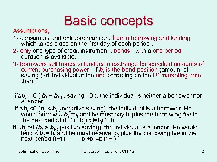Basic concepts Assumptions; 1 - consumers and entrepreneurs are free in borrowing and lending which takes place on the first day of each period. 2 - only one type of credit instrument , bonds , with a one period duration is available. 3 - borrowers sell bonds to lenders in exchange for specified amounts of current purchasing power. If bt is the bond position (amount of saving ) of individual at the end of trading on the t th marketing date, then if∆bt = 0 ( bt = bt-1 , saving =0 ), the individual is neither a borrower nor a lender if ∆bt <0 (bt < bt-1 negative saving), the individual is a borrower. He would borrow ∆ bt =bt and he must pay bt plus the borrowing fee in the next period (t+1). bt+bti=bt(1+i) if ∆bt >0 (bt > bt-1 positive saving), the individual is a lender. He would lend ∆ bt = bt and he must receive bt plus the borrowing fee in the next period (t+1). bt+bti=bt(1+i) optimization over time Henderson , Quandt , CH 12 2

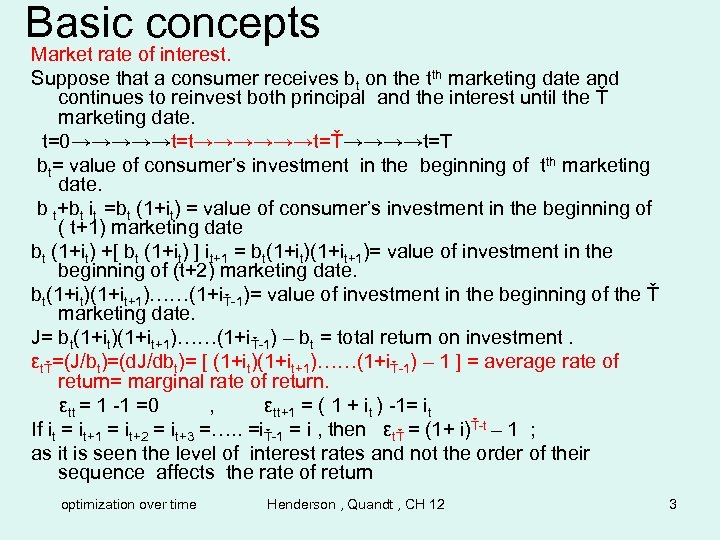Basic concepts Market rate of interest. Suppose that a consumer receives bt on the tth marketing date and continues to reinvest both principal and the interest until the Ť marketing date. t=0→→→→→t=t→→→→→→t=Ť→→→→t=T bt= value of consumer’s investment in the beginning of tth marketing date. b t+bt it =bt (1+it) = value of consumer’s investment in the beginning of ( t+1) marketing date bt (1+it) +[ bt (1+it) ] it+1 = bt(1+it)(1+it+1)= value of investment in the beginning of (t+2) marketing date. bt(1+it)(1+it+1)……(1+iŤ-1)= value of investment in the beginning of the Ť marketing date. J= bt(1+it)(1+it+1)……(1+iŤ-1) – bt = total return on investment. εtŤ=(J/bt)=(d. J/dbt)= [ (1+it)(1+it+1)……(1+iŤ-1) – 1 ] = average rate of return= marginal rate of return. εtt = 1 -1 =0 , εtt+1 = ( 1 + it ) -1= it If it = it+1 = it+2 = it+3 =…. . =iŤ-1 = i , then εtŤ = (1+ i)Ť-t – 1 ; as it is seen the level of interest rates and not the order of their sequence affects the rate of return optimization over time Henderson , Quandt , CH 12 3

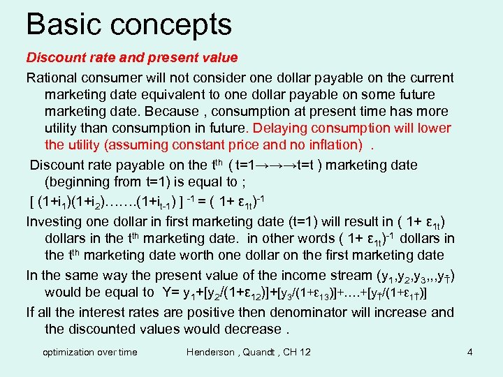Basic concepts Discount rate and present value Rational consumer will not consider one dollar payable on the current marketing date equivalent to one dollar payable on some future marketing date. Because , consumption at present time has more utility than consumption in future. Delaying consumption will lower the utility (assuming constant price and no inflation). Discount rate payable on the tth ( t=1→→→t=t ) marketing date (beginning from t=1) is equal to ; [ (1+i 1)(1+i 2)……. (1+it-1) ] -1 = ( 1+ ε 1 t)-1 Investing one dollar in first marketing date (t=1) will result in ( 1+ ε 1 t) dollars in the tth marketing date. in other words ( 1+ ε 1 t)-1 dollars in the tth marketing date worth one dollar on the first marketing date In the same way the present value of the income stream (y 1, y 2, y 3, , , yŤ) would be equal to Y= y 1+[y 2/(1+ε 12)]+[y 3/(1+ε 13)]+…. +[yŤ/(1+ε 1Ť)] If all the interest rates are positive then denominator will increase and the discounted values would decrease. optimization over time Henderson , Quandt , CH 12 4

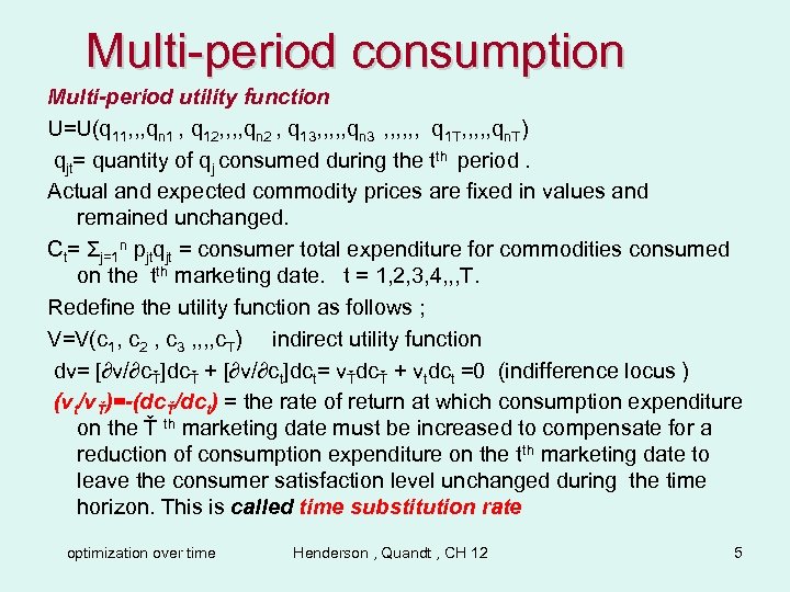Multi-period consumption Multi-period utility function U=U(q 11, , , qn 1 , q 12, , qn 2 , q 13, , , qn 3 , , , q 1 T, , , qn. T) qjt= quantity of qj consumed during the tth period. Actual and expected commodity prices are fixed in values and remained unchanged. Ct= Σj=1 n pjtqjt = consumer total expenditure for commodities consumed on the tth marketing date. t = 1, 2, 3, 4, , , T. Redefine the utility function as follows ; V=V(c 1, c 2 , c 3 , , c. T) indirect utility function dv= [∂v/∂cŤ]dcŤ + [∂v/∂ct]dct= vŤdcŤ + vtdct =0 (indifference locus ) (vt/vŤ)=-(dcŤ/dct) = the rate of return at which consumption expenditure on the Ť th marketing date must be increased to compensate for a reduction of consumption expenditure on the tth marketing date to leave the consumer satisfaction level unchanged during the time horizon. This is called time substitution rate optimization over time Henderson , Quandt , CH 12 5

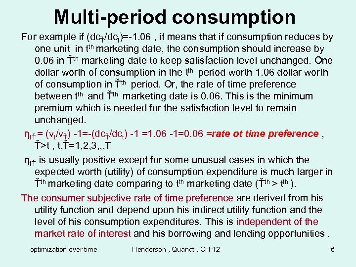Multi-period consumption For example if (dcŤ/dct)=-1. 06 , it means that if consumption reduces by one unit in tth marketing date, the consumption should increase by 0. 06 in Ťth marketing date to keep satisfaction level unchanged. One dollar worth of consumption in the tth period worth 1. 06 dollar worth of consumption in Ťth period. Or, the rate of time preference between tth and Ťth marketing date is 0. 06. This is the minimum premium which is needed for the satisfaction level to remain unchanged. ηtŤ = (vt/vŤ) -1=-(dcŤ/dct) -1 =1. 06 -1=0. 06 =rate ot time preference , Ť>t , t, Ť=1, 2, 3, , , T ηtŤ is usually positive except for some unusual cases in which the expected worth (utility) of consumption expenditure is much larger in Ťth marketing date comparing to tth marketing date (Ťth > tth ). The consumer subjective rate of time preference are derived from his utility function and depend upon his indirect utility function and the level of his consumption expenditures. This is independent of the market rate of interest and his borrowing and lending opportunities. optimization over time Henderson , Quandt , CH 12 6

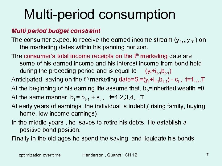Multi-period consumption Multi period budget constraint The consumer expect to receive the earned income stream (y 1, , , y Ť ) on the marketing dates within his panning horizon. The consumer’s total income receipts on the tth marketing date are some of his earned income and his interest income from bond held during the preceding period and is equal to (yt+it-1 bt-1) Anticipated saving on the tth marketing date=St=(yt+it-1 bt-1) - ct , t=1, , T At the beginning of his earning life assume that, b 0=inherited wealth =0 At the same manner bt = bt-1 + st , t=1, 2, 3, 4, , T. At early years of earnings , the individual is indebt, ( rising family, buying home, low income earnings) In the middle years , he saves to retire his debts. He establish a positive bond position. Finally in the old ages he spend the saving and liquidate his bonds optimization over time Henderson , Quandt , CH 12 7

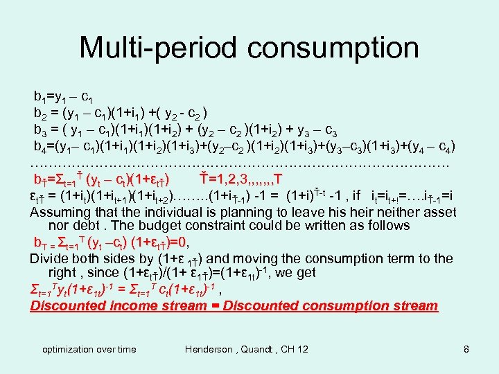Multi-period consumption b 1=y 1 – c 1 b 2 = (y 1 – c 1)(1+i 1) +( y 2 - c 2 ) b 3 = ( y 1 – c 1)(1+i 2) + (y 2 – c 2 )(1+i 2) + y 3 – c 3 b 4=(y 1– c 1)(1+i 2)(1+i 3)+(y 2–c 2 )(1+i 2)(1+i 3)+(y 3–c 3)(1+i 3)+(y 4 – c 4) ………………………………………. bŤ=Σt=1Ť (yt – ct)(1+εtŤ) Ť=1, 2, 3, , , , T εtŤ = (1+it)(1+it+1)(1+it+2)……. . (1+iŤ-1) -1 = (1+i)Ť-t -1 , if it=it+!=…. iŤ-1=i Assuming that the individual is planning to leave his heir neither asset nor debt. The budget constraint could be written as follows b. T = Σt=1 T (yt –ct) (1+εtŤ)=0, )=0 Divide both sides by (1+ε 1Ť) and moving the consumption term to the right , since (1+εtŤ)/(1+ ε 1Ť)=(1+ε 1 t)-1, we get Σt=1 Tyt(1+ε 1 t)-1 = Σt=1 T ct(1+ε 1 t)-1 , Discounted income stream = Discounted consumption stream optimization over time Henderson , Quandt , CH 12 8

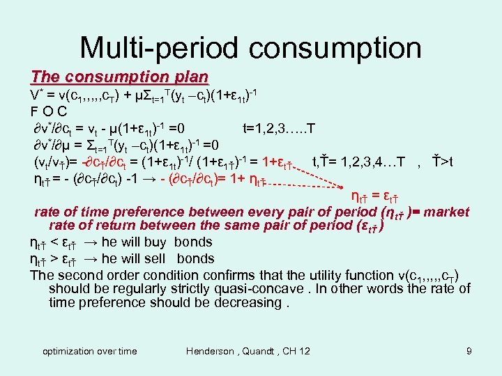Multi-period consumption The consumption plan V* = v(c 1, , , c. T) + µΣt=1 T(yt –ct)(1+ε 1 t)-1 FOC ∂v*/∂ct = vt - µ(1+ε 1 t)-1 =0 t=1, 2, 3…. . T ∂v*/∂µ = Σt=1 T(yt –ct)(1+ε 1 t)-1 =0 (vt/vŤ)= -∂cŤ/∂ct = (1+ε 1 t)-1/ (1+ε 1Ť)-1 = 1+εtŤ t, Ť= 1, 2, 3, 4…T , Ť>t ηtŤ = - (∂cŤ/∂ct) -1 → - (∂cŤ/∂ct)= 1+ ηtŤ = εtŤ rate of time preference between every pair of period (ηtŤ )= market rate of return between the same pair of period (εtŤ ) ηtŤ < εtŤ → he will buy bonds ηtŤ > εtŤ → he will sell bonds The second order condition confirms that the utility function v(c 1, , , c. T) should be regularly strictly quasi-concave. In other words the rate of time preference should be decreasing. optimization over time Henderson , Quandt , CH 12 9

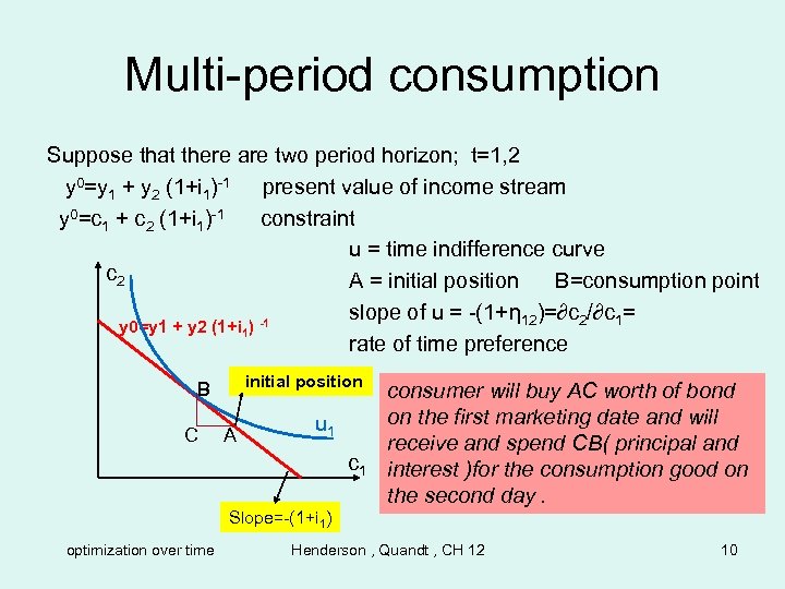Multi-period consumption Suppose that there are two period horizon; t=1, 2 y 0=y 1 + y 2 (1+i 1)-1 present value of income stream y 0=c 1 + c 2 (1+i 1)-1 constraint u = time indifference curve c 2 A = initial position B=consumption point slope of u = -(1+η 12)=∂c 2/∂c 1= y 0=y 1 + y 2 (1+i 1) -1 rate of time preference initial position B C A u 1 consumer will buy AC worth of bond on the first marketing date and will receive and spend CB( principal and interest )for the consumption good on the second day. Slope=-(1+i 1) optimization over time Henderson , Quandt , CH 12 10

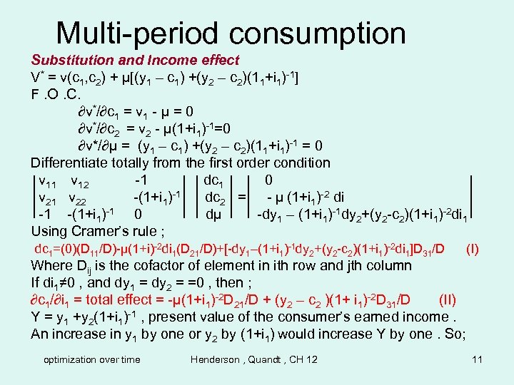Multi-period consumption Substitution and Income effect V* = v(c 1, c 2) + µ[(y 1 – c 1) +(y 2 – c 2)(11+i 1)-1] F. O. C. ∂v*/∂c 1 = v 1 - µ = 0 ∂v*/∂c 2 = v 2 - µ(1+i 1)-1=0 ∂v*/∂µ = (y 1 – c 1) +(y 2 – c 2)(11+i 1)-1 = 0 Differentiate totally from the first order condition v 11 v 12 -1 dc 1 0 v 21 v 22 -(1+i 1)-1 dc 2 = - µ (1+i 1)-2 di -1 -(1+i 1)-1 0 dµ -dy 1 – (1+i 1)-1 dy 2+(y 2 -c 2)(1+i 1)-2 di 1 Using Cramer’s rule ; dc 1=(0)(D 11/D)-µ(1+i)-2 di 1(D 21/D)+[-dy 1–(1+i 1)-1 dy 2+(y 2 -c 2)(1+i 1)-2 di 1]D 31/D (I) Where Dij is the cofactor of element in ith row and jth column If di 1≠ 0 , and dy 1 = dy 2 = =0 , then ; ∂c 1/∂i 1 = total effect = -µ(1+i 1)-2 D 21/D + (y 2 – c 2 )(1+ i 1)-2 D 31/D (II) Y = y 1 +y 2(1+i 1)-1 , present value of the consumer’s earned income. An increase in y 1 by one or y 2 by (1+i 1) would increase Y by one. So; optimization over time Henderson , Quandt , CH 12 11

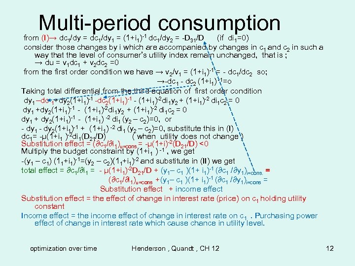Multi-period consumption from (I)→ dc 1/dy = dc 1/dy 1 = (1+i 1)-1 dc 1/dy 2 = -D 31/D (if di 1=0) consider those changes by i which are accompanied by changes in c 1 and c 2 in such a way that the level of consumer’s utility index remain unchanged, that is ; → du = v 1 dc 1 + v 2 dc 2 =0 from the first order condition we have → v 2/v 1 = (1+i 1)-1 = - dc 1/dc 2 so; →-dc 1 - dc 2 (1+i 1) -1=o Taking total differential from the third equation of first order condition dy 1 –dc 1+dy 2(1+i 1)-1 -dc 2(1+i 1)-1 - (1+i 1)-2 di 1 y 2 + (1+i 1)-2 di 1 c 2 = 0 dy 1 +dy 2(1+i 1)-1 - (1+i 1)-2 di 1 y 2 + (1+i 1)-2 di 1 c 2 = 0 dy 1 + dy 2(1+i 1)-1 - (1+i 1) -2 di 1 (y 2 – c 2)=0, or - dy 1 - dy 2(1+i 1)-1 + (1+i 1) -2 di 1 (y 2 – c 2)=0, substitute this in (I) dc 1= -µ(1+i 1 )-2 di 1(D 21/D) ( when utility does not change ) Substitution effect = (∂c 1/∂i 1)u=cons. = -µ(1+i)-2(D 21/D) <0 Multiply the budget constraint by (1+i 1 ) -1 , we get -(y 1 – c 1) (11+i 1)-1=(y 2 – c 2)(11+i 1)-2 and substitute in (II) we get total effect = ∂c 1/∂i 1 = - µ(1+i 1)-2 D 21/D + (y 1– c 1 )(1+ i 1)-1 (∂c 1 /∂y 1)i=cons. = (∂c 1/∂i 1)u=cons +(y 1– c 1 )(1+ i 1)-1 (∂c 1 /∂y 1)i=cons = Substitution effect + income effect Substitution effect = the effect of change in interest rate (price) on c 1 holding utility constant Income effect = the income effect of change in interest rate on c 1. Purchasing power effect of change in interest rate which cause chance in utility level. optimization over time Henderson , Quandt , CH 12 12

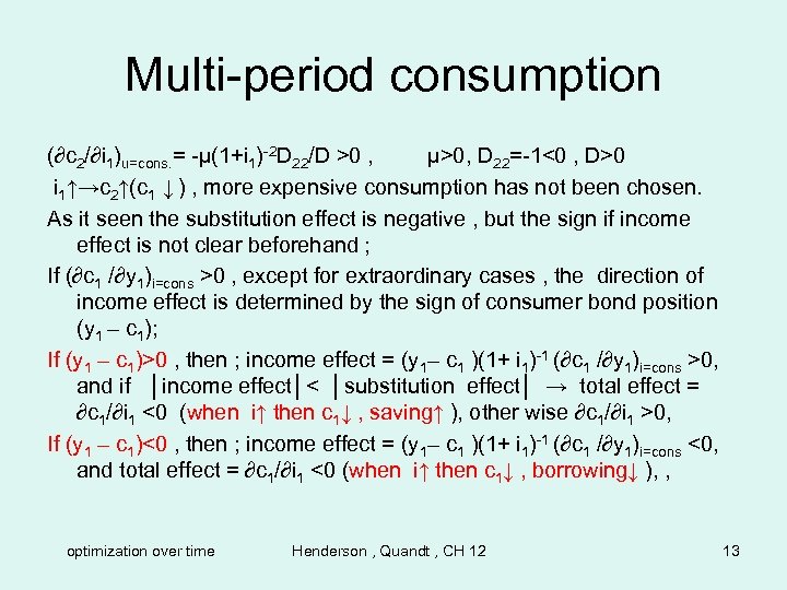Multi-period consumption (∂c 2/∂i 1)u=cons. = -µ(1+i 1)-2 D 22/D >0 , µ>0, D 22=-1<0 , D>0 i 1↑→c 2↑(c 1 ↓ ) , more expensive consumption has not been chosen. As it seen the substitution effect is negative , but the sign if income effect is not clear beforehand ; If (∂c 1 /∂y 1)i=cons >0 , except for extraordinary cases , the direction of income effect is determined by the sign of consumer bond position (y 1 – c 1); If (y 1 – c 1)>0 , then ; income effect = (y 1– c 1 )(1+ i 1)-1 (∂c 1 /∂y 1)i=cons >0, and if │income effect│< │substitution effect│ → total effect = ∂c 1/∂i 1 <0 (when i↑ then c 1↓ , saving↑ ), other wise ∂c 1/∂i 1 >0, If (y 1 – c 1)<0 , then ; income effect = (y 1– c 1 )(1+ i 1)-1 (∂c 1 /∂y 1)i=cons <0, and total effect = ∂c 1/∂i 1 <0 (when i↑ then c 1↓ , borrowing↓ ), , optimization over time Henderson , Quandt , CH 12 13

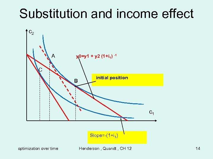Substitution and income effect c 2 A y 0=y 1 + y 2 (1+i 1) -1 C B initial position c 1 Slope=-(1+i 1) optimization over time Henderson , Quandt , CH 12 14

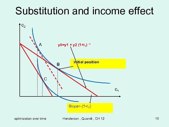Substitution and income effect c 2 A y 0=y 1 + y 2 (1+i 1) -1 B initial position C c 1 Slope=-(1+i 1) optimization over time Henderson , Quandt , CH 12 15

Investment theory of the firm Generally time must elapse between the application of inputs and securing the inputs. There are few assumptions ; 1 - the entrepreneurs buys input and sells output only on marketing dates within his horizon. 2 - he performs the technical operation of his production process in the time between marketing dates. 3 - during the period t , he applies the inputs he has bought on the t th marketing dates. 4 - on the (t+1) th marketing date he sells the output which he secured during the t th period. 5 - input and output prices are fixed , so investment expenditures and revenues from sale on each of the marketing dates acts as decision variables. optimization over time Henderson , Quandt , CH 12 16

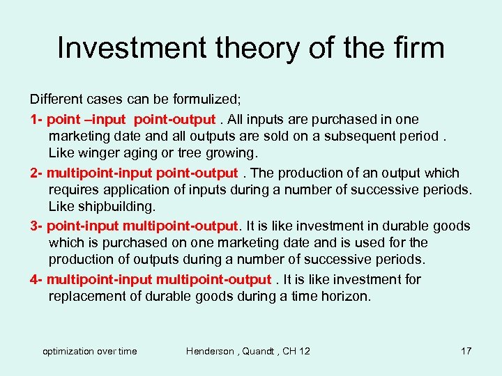Investment theory of the firm Different cases can be formulized; 1 - point –input point-output. All inputs are purchased in one marketing date and all outputs are sold on a subsequent period. Like winger aging or tree growing. 2 - multipoint-input point-output. The production of an output which requires application of inputs during a number of successive periods. Like shipbuilding. 3 - point-input multipoint-output. It is like investment in durable goods which is purchased on one marketing date and is used for the production of outputs during a number of successive periods. 4 - multipoint-input multipoint-output. It is like investment for replacement of durable goods during a time horizon. optimization over time Henderson , Quandt , CH 12 17

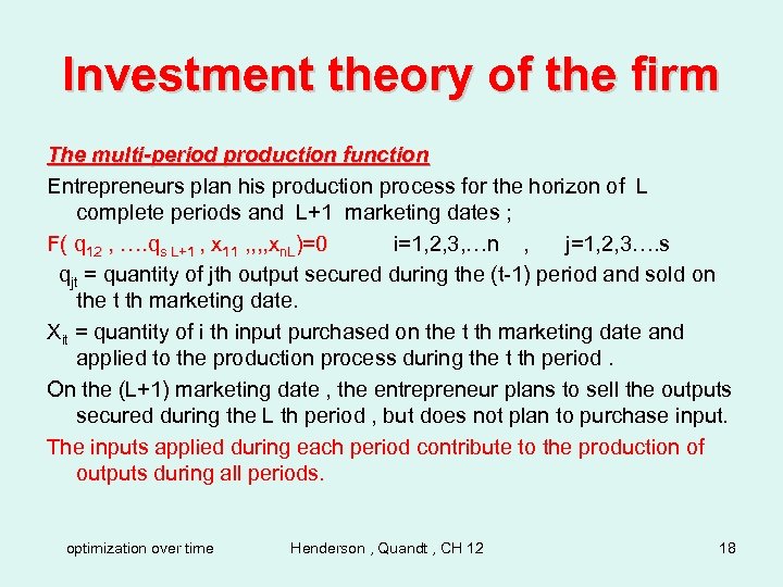Investment theory of the firm The multi-period production function Entrepreneurs plan his production process for the horizon of L complete periods and L+1 marketing dates ; F( q 12 , …. qs L+1 , x 11 , , xn. L)=0 i=1, 2, 3, …n , j=1, 2, 3…. s qjt = quantity of jth output secured during the (t-1) period and sold on the t th marketing date. Xit = quantity of i th input purchased on the t th marketing date and applied to the production process during the t th period. On the (L+1) marketing date , the entrepreneur plans to sell the outputs secured during the L th period , but does not plan to purchase input. The inputs applied during each period contribute to the production of outputs during all periods. optimization over time Henderson , Quandt , CH 12 18

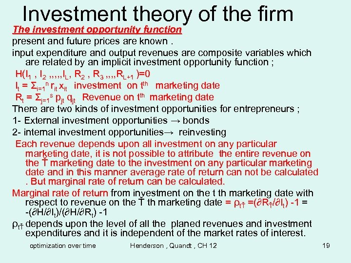Investment theory of the firm The investment opportunity function present and future prices are known. input expenditure and output revenues are composite variables which are related by an implicit investment opportunity function ; H(I 1 , I 2 , , , IL, R 2 , R 3 , , RL+1 )=0 It = Σi=1 n rit xit investment on tth marketing date Rt = Σj=1 s pjt qjt Revenue on tth marketing date There are two kinds of investment opportunities for entrepreneurs ; 1 - External investment opportunities → bonds 2 - internal investment opportunities→ reinvesting Each revenue depends upon all investment on any particular marketing date, it is not possible to attribute the entire revenue on the Ť marketing date to the investment on any particular marketing date and in this manner average rate of return can not be calculated. But marginal rate of return can be calculated. Marginal rate of return from investment on the t th marketing date with respect to revenue on the Ť th marketing date = ρtŤ =(∂RŤ/∂It) -1 = -(∂H/∂It)/(∂H/∂Rt) -1 ρtŤ depends upon the level of all the planed revenues and investment expenditures and it is independent of the market rates of interest. optimization over time Henderson , Quandt , CH 12 19

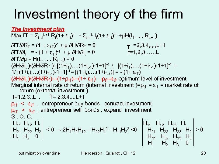Investment theory of the firm The investment plan Max Π* = Σt=2 L+1 Rt(1+ ε 1 t)-1 - Σt=1 L It(1+ ε 1 t)-1 +µH(I 1, , , RL+1) ∂Π*/∂RŤ = (1 + ε 1Ť)-1 + µ ∂H/∂RŤ = 0 Ť =2, 3, 4, , , L+1 ∂Π*/∂It = - (1 + ε 1 t)-1 + µ ∂H/∂It = 0 t=1, 2, 3……L ∂Π*/∂µ = H(I 1, , , RL+1) = 0 (∂H/∂It )/(∂H/∂RŤ )=[(1+i 1)…. (1+it-1)-1+1]-1 / [(1+i 1)…. (1+iŤ-1)-1+1]-1 = 1/ [(1+it)…. (1+iŤ-1)-1+1]-1= [(1+it)…. (1+iŤ-1)] = - (1+ εtŤ) (∂H/∂It )/(∂H/∂RŤ)=-(1+ρtŤ)=-(1+ εtŤ) →ρtŤ=εtŤ optimum level of investment Marginal internal rate of return (internal investment )=ρtŤ = εtŤ = market rate of return (external investment ) t=1, 2, 3. . L , Ť= 2, 3, 4, , L+1 ρtŤ < εtŤ , entrepreneur buy bonds , contract investment ρtŤ > εtŤ , entrepreneur sell bonds , expand investment S. O. C. H 11 H 12 H 13 H 1 H 22 H 2 < 0 → 2 H 1 H 2 H 12 – H 22 H 12 – H 11 H 22 <0 H 21 H 22 H 23 H 2 > 0 H 1 H 2 0 H 31 H 32 H 33 H 1 H 2 H 3 0 optimization over time Henderson , Quandt , CH 12 20

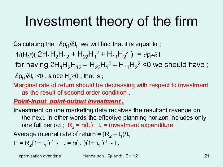Investment theory of the firm Calculating the ∂ρtŤ/∂It we will find that it is equal to ; -1/(H 23)(-2 H 1 H 2 H 12 + H 22 H 12 + H 11 H 22 ) = ∂ρtŤ/∂It for having 2 H 1 H 2 H 12 – H 22 H 12 – H 11 H 22 <0 we should have ; ∂ρtŤ/∂It <0 , since H 2>0 , that is ; Marginal rate of return should be decreasing with respect to investment as the result of second order condition. Point-input point-output investment. Investment on one marketing date receives the resultant revenue on the next. In other words the effective planning horizon includes only one full period ; R 2 = h(I 1) I 1 = investment expenditure Average internal rate of return = (R 2 – I 1)/I 1 Π = R 2(1+ i 1 )-1 - I 1 = h(I 1 )(1+ i 1 )-1 - I 1 optimization over time Henderson , Quandt , CH 12 21

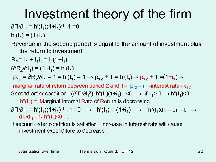Investment theory of the firm ∂Π/∂I 1 = h’(I 1)(1+i 1)-1 -1 =0 h’(I 1) = (1+i 1) Revenue in the second period is equal to the amount of investment plus the return to investment. R 2 = I 1 + I 1 i 1 = I 1(1+i 1) (∂R 2/∂I 1) = (1+i 1) = h’(I 1) ρ12 = ∂R 2/∂I 1 – 1 = h’(I 1) – 1 → ρ12 + 1 = h’(I 1)→ ρ12 + 1 =(1+i 1)→ marginal rate of return between period 2 and 1= ρ12 = i 1 =interest rate= ε 12 Second order condition ; (∂2Π/∂I 12)=h”(I 1)(1+i 1)-1 <0 → if i 1> 0 → h”(I 1)<0 h”(I 1) = Marginal Internal Rate of Return is decreasing. ∂Π/∂I 1 = h’(I 1)(1+i 1)-1 -1 =0 → h’(I 1) = (1+i 1) → h”(I 1)d. I 1 – di 1 =0 → d. I 1/di 1 =1/ h”(I 1)<0 , If second order condition is satisfied , increase in interest rate will cause investment expenditure to decrease. optimization over time Henderson , Quandt , CH 12 22

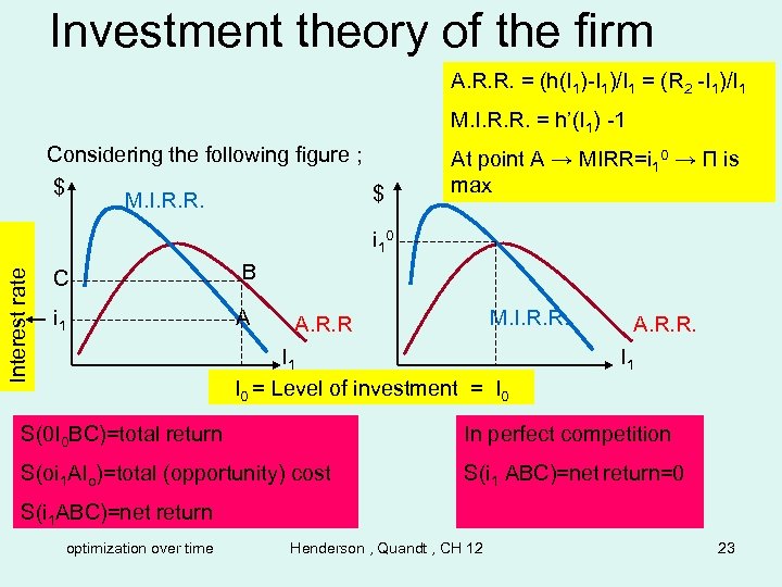Investment theory of the firm A. R. R. = (h(I 1)-I 1)/I 1 = (R 2 -I 1)/I 1 M. I. R. R. = h’(I 1) -1 Considering the following figure ; $ $ M. I. R. R. At point A → MIRR=i 10 → Π is max Interest rate i 1 0 C B i 1 A M. I. R. R. A. R. R I 1 I 0 = Level of investment = I 1 I 0 0 0 A. R. R. I 1 S(0 I 0 BC)=total return In perfect competition S(oi 1 AIo)=total (opportunity) cost S(i 1 ABC)=net return=0 S(i 1 ABC)=net return optimization over time Henderson , Quandt , CH 12 23

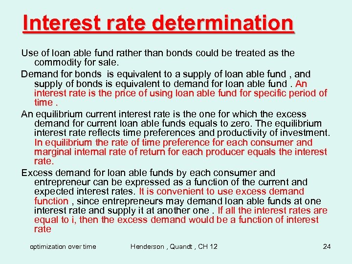Interest rate determination Use of loan able fund rather than bonds could be treated as the commodity for sale. Demand for bonds is equivalent to a supply of loan able fund , and supply of bonds is equivalent to demand for loan able fund. An interest rate is the price of using loan able fund for specific period of time. An equilibrium current interest rate is the one for which the excess demand for current loan able funds equals to zero. The equilibrium interest rate reflects time preferences and productivity of investment. In equilibrium the rate of time preference for each consumer and marginal internal rate of return for each producer equals the interest rate. Excess demand for loan able funds by each consumer and entrepreneur can be expressed as a function of the current and expected interest rates. It is convenient to use excess demand function , since entrepreneurs may demand loan able funds at one interest rate and supply it at another one. If all the interest rates are equal to i, then the excess demand would be a function of interest rate optimization over time Henderson , Quandt , CH 12 24

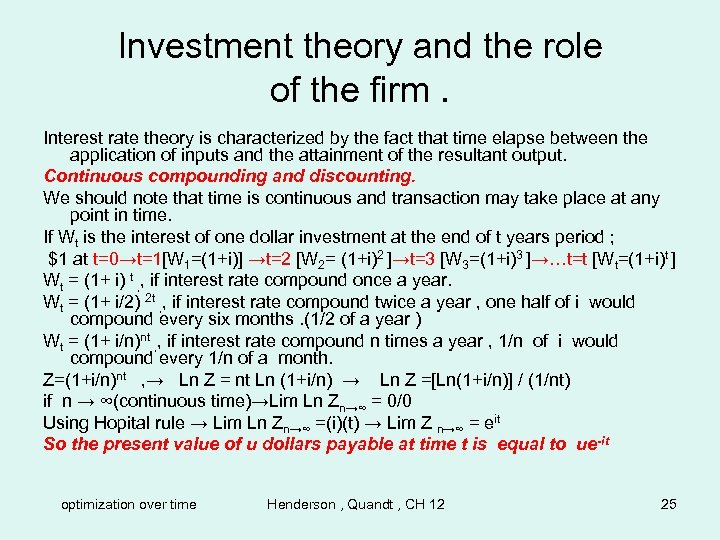Investment theory and the role of the firm. Interest rate theory is characterized by the fact that time elapse between the application of inputs and the attainment of the resultant output. Continuous compounding and discounting. We should note that time is continuous and transaction may take place at any point in time. If Wt is the interest of one dollar investment at the end of t years period ; $1 at t=0→t=1[W 1=(1+i)] →t=2 [W 2= (1+i)2 ]→t=3 [W 3=(1+i)3 ]→…t=t [Wt=(1+i)t ] Wt = (1+ i) t , , if interest rate compound once a year. Wt = (1+ i/2) 2 t , , if interest rate compound twice a year , one half of i would compound every six months. (1/2 of a year ) Wt = (1+ i/n)nt , , if interest rate compound n times a year , 1/n of i would compound every 1/n of a month. Z=(1+i/n)nt , → Ln Z = nt Ln (1+i/n) → Ln Z =[Ln(1+i/n)] / (1/nt) if n → ∞(continuous time)→Lim Ln Zn→∞ = 0/0 Using Hopital rule → Lim Ln Zn→∞ =(i)(t) → Lim Z n→∞ = eit So the present value of u dollars payable at time t is equal to ue -it optimization over time Henderson , Quandt , CH 12 25

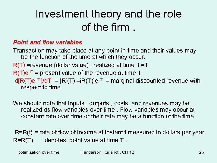Investment theory and the role of the firm. Point and flow variables Transaction may take place at any point in time and their values may be the function of the time at which they occur. R(T) =revenue (dollar value) , realized at time t =T R(T)e-i. T = present value of the revenue at time T d[R(T)e-i. T ]/d. T = [R’(T) –i. R(T)]e-i. T = marginal discounted revenue with respect to time. We should note that inputs , outputs , costs, and revenues may be realized as flow variables over time. Flow variables may occur at constant rate over time or their rate may be a function of the time. R=R(t) = rate of flow of income at instant t measured in dollars per year. R=R(T) denotes point value at time T. optimization over time Henderson , Quandt , CH 12 26

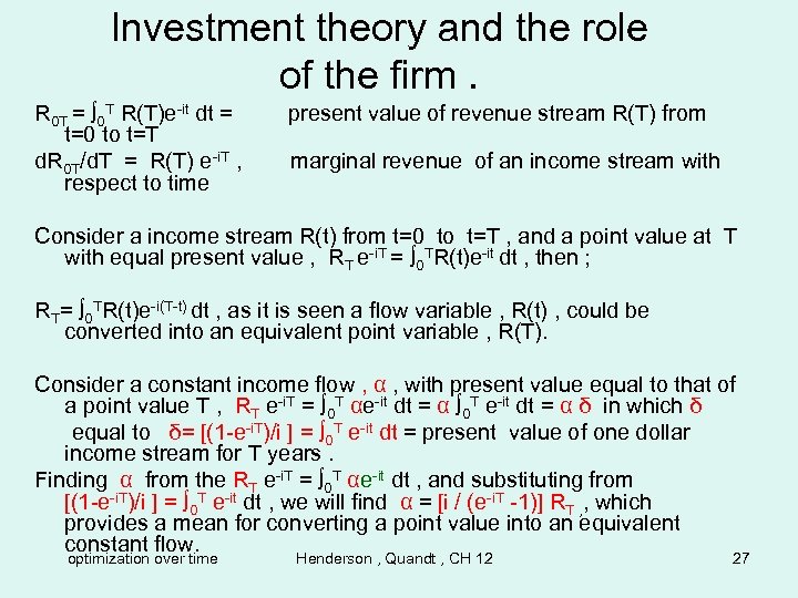Investment theory and the role of the firm. R 0 T = ∫ 0 T R(T)e-it dt = t=0 to t=T d. R 0 T/d. T = R(T) e-i. T , respect to time present value of revenue stream R(T) from marginal revenue of an income stream with Consider a income stream R(t) from t=0 to t=T , and a point value at T with equal present value , RT e-i. T = ∫ 0 TR(t)e-it dt , then ; RT= ∫ 0 TR(t)e-i(T-t) dt , as it is seen a flow variable , R(t) , could be converted into an equivalent point variable , R(T). Consider a constant income flow , α , with present value equal to that of a point value T , RT e-i. T = ∫ 0 T αe-it dt = α ∫ 0 T e-it dt = α δ in which δ equal to δ= [(1 -e-i. T)/i ] = ∫ 0 T e-it dt = present value of one dollar income stream for T years. Finding α from the RT e-i. T = ∫ 0 T αe-it dt , and substituting from [(1 -e-i. T)/i ] = ∫ 0 T e-it dt , we will find α = [i / (e-i. T -1)] RT , , which provides a mean for converting a point value into an equivalent constant flow. optimization over time Henderson , Quandt , CH 12 27

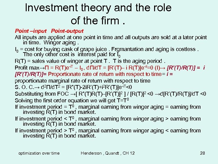Investment theory and the role of the firm. Point –input Point-output All inputs are applied at one point in time and all outputs are sold at a later point in time. Winger aging. I 0 = cost for buying cask of grape juice. Frgmantation and aging is costless. The only other cost is interest paid for I 0 R(T) = sales value of winger at point T. T is the aging period. Profit max→Π = R(T)e-i. T – I 0 , dΠ/d. T = [R’(T)– i R(T)]e-it=0 (I)→ [R’(T)/R(T)] = i [R’(T)/R(T)]= Proportionate rate of return with respect to time= i = proportionate marginal rate of return with respect to time S. O. C. → d 2Π/d. T 2 = [R”(T)-2 i. R’(T)+i 2 R’(T)]e-i. T<0 Substituting from FOC →[ R”(T)R(T)–[R’(T)]2 ] / [R(T)]2 <0 →d[R’(T)/R(T)]/d. T <0 Solving the first order equation we will get T=T 0 If investment period = T 0 , marginal earning from winger aging = earning from investing R(T) in bond market. If investment period < T 0 , marginal earning from winger aging > earning from investing R(T) in bond market. If investment period > T 0 , marginal earning from winger aging < earning from investing R(T) in bond market. optimization over time Henderson , Quandt , CH 12 28

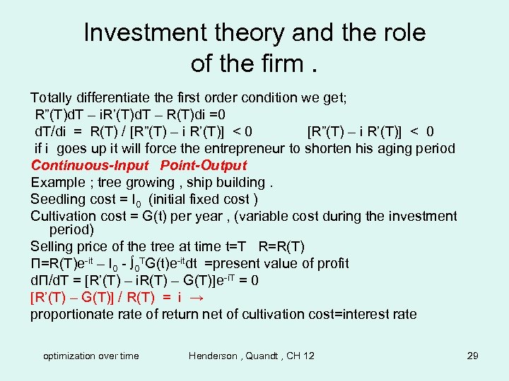Investment theory and the role of the firm. Totally differentiate the first order condition we get; R”(T)d. T – i. R’(T)d. T – R(T)di =0 d. T/di = R(T) / [R”(T) – i R’(T)] < 0 if i goes up it will force the entrepreneur to shorten his aging period Continuous-Input Point-Output Example ; tree growing , ship building. Seedling cost = I 0 (initial fixed cost ) Cultivation cost = G(t) per year , (variable cost during the investment period) Selling price of the tree at time t=T R=R(T) Π=R(T)e-it – I 0 - ∫ 0 TG(t)e-itdt =present value of profit dΠ/d. T = [R’(T) – i. R(T) – G(T)]e-i. T = 0 [R’(T) – G(T)] / R(T) = i → proportionate rate of return net of cultivation cost=interest rate optimization over time Henderson , Quandt , CH 12 29

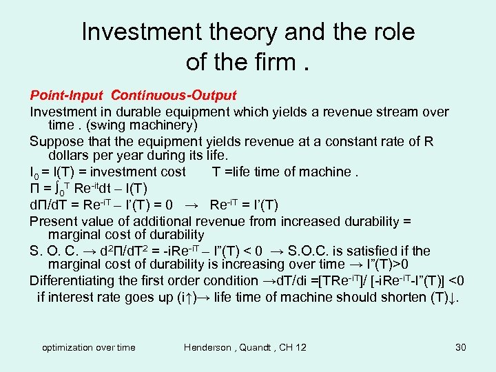Investment theory and the role of the firm. Point-Input Continuous-Output Investment in durable equipment which yields a revenue stream over time. (swing machinery) Suppose that the equipment yields revenue at a constant rate of R dollars per year during its life. I 0 = I(T) = investment cost T =life time of machine. Π = ∫ 0 T Re-itdt – I(T) dΠ/d. T = Re-i. T – I’(T) = 0 → Re-i. T = I’(T) Present value of additional revenue from increased durability = marginal cost of durability S. O. C. → d 2Π/d. T 2 = -i. Re-i. T – I”(T) < 0 → S. O. C. is satisfied if the marginal cost of durability is increasing over time → I”(T)>0 Differentiating the first order condition →d. T/di =[TRe-i. T]/ [-i. Re-i. T-I”(T)] <0 if interest rate goes up (i↑)→ life time of machine should shorten (T)↓. optimization over time Henderson , Quandt , CH 12 30

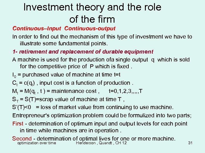Investment theory and the role of the firm Continuous–Input Continuous-output In order to find out the mechanism of this type of investment we have to illustrate some fundamental points. 1 - retirement and replacement of durable equipment A machine is used for the production ofa single output q which is sold for the competitive price of P which is fixed. I 0 = purchased value of machine at time t=t Ct = c(qt) , input cost is a function of production. Mt = M(qt , t ) = maintenance cost , t=0, 1, 2, 3, , , T ST = S(T)=scrap value of machine at time T , S’(T)<0 = loss of market value from continuing to use machine. Entrepreneur's optimization problem could be formulized into two parts; First - determination of optimum input and output levels for each point in time while machines are in operation. Second - determination of optimal lives for one or more machine. optimization over time Henderson , Quandt , CH 12 31

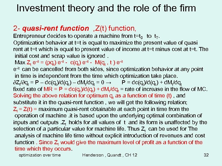Investment theory and the role of the firm 2 - quasi-rent function , Z(t) function, Entrepreneur decides to operate a machine from t=t 0 to t. T. Optimization behavior at t=t is equal to maximize the present value of quasi rent at t=t which is equal to present value of income at t=t minus cost at t=t. The initial cost and scrap value is ignored. Max Zt e-it = (pqt) e-it - c(qt) e-it - M(qt , t ) e-it can be cancelled from both sides, since optimization behavior at any point in time is independent from the time which optimization take place. ∂Zt/∂qt = P – dc(qt)/d(qt) – d. Mt/dqt = 0 → P = dc(qt)/d(qt) + d. Mt/dqt fixed rate of MR = P = dc(qt)/d(qt) + d. Mt/dqt = rate of increase in the flow of MC. Solving the above relation for optimum qt as a function of time (t) , and substitute it in the quasi-rent function , we will get the following relation; Zt = Z(t) = maximum quasi-rent obtainable at each point in time from the operation of machine. it is based upon the underlying optimal combination of inputs and outputs. Zt holds for all values of t and its form is unaffected by the selection of a particular value for machine life. Thus Zt can be used for The analysis of machine life time without explicit introduction of revenues and cost function. Since Zt would give the maximum level of profit as a function of the time which they occurs. optimization over time Henderson , Quandt , CH 12 32

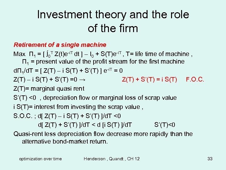Investment theory and the role of the firm Retirement of a single machine Max Π 1 = [ ∫ 0 T Z(t)e-i. T dt ] – I 0 + S(T)e-i. T , T= life time of machine , Π 1 = present value of the profit stream for the first machine dΠ 1/d. T = [ Z(T) – i S(T) + S’(T) ] e-i. T = 0 Z(T) – i S(T) + S’(T) =0 → Z(T) + S’(T) = i S(T) F. O. C. Z(T)= marginal quasi rent S’(T) <0 , depreciation flow or marginal loss of scrap value i S(T)= interest from investing the scrap value , S. O. C. ; d[ Z(T) – i S(T) + S’(T) ]/d. T <0 d[ Z(T) + S’(T) ]/d. T < d [i S(T) ]/d. T S’(T)<0 Quasi-rent less depreciation flow decrease more rapidly than the alternative bond-market return. optimization over time Henderson , Quandt , CH 12 33

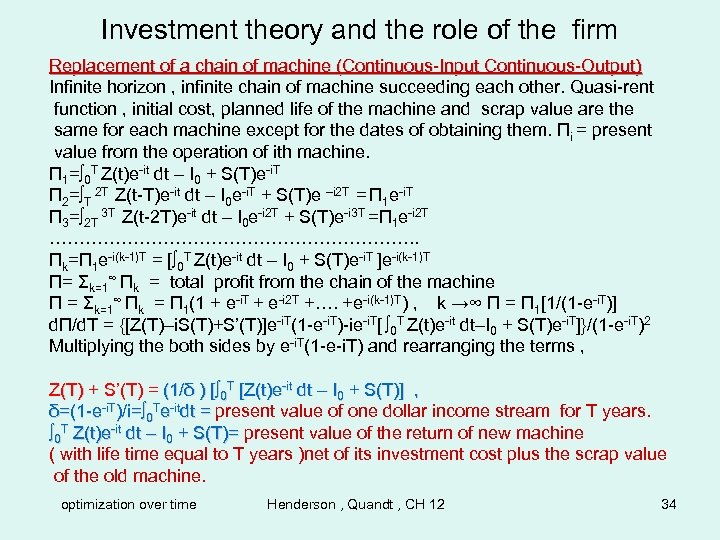Investment theory and the role of the firm Replacement of a chain of machine (Continuous-Input Continuous-Output) Infinite horizon , infinite chain of machine succeeding each other. Quasi-rent function , initial cost, planned life of the machine and scrap value are the same for each machine except for the dates of obtaining them. Πi = present value from the operation of ith machine. Π 1=∫ 0 T Z(t)e-it dt – I 0 + S(T)e-i. T Π 2=∫T 2 T Z(t-T)e-it dt – I 0 e-i. T + S(T)e –i 2 T = Π 1 e-i. T Π 3=∫ 2 T 3 T Z(t-2 T)e-it dt – I 0 e-i 2 T + S(T)e-i 3 T =Π 1 e-i 2 T …………………………. . Πk=Π 1 e-i(k-1)T = [∫ 0 T Z(t)e-it dt – I 0 + S(T)e-i. T ]e-i(k-1)T Π= Σk=1∞ Πk = total profit from the chain of the machine Π = Σk=1∞ Πk = Π 1(1 + e-i. T + e-i 2 T +…. +e-i(k-1)T) , k →∞ Π = Π 1[1/(1 -e-i. T)] dΠ/d. T = {[Z(T)–i. S(T)+S’(T)]e-i. T(1 -e-i. T)-ie-i. T[ ∫ 0 T Z(t)e-it dt–I 0 + S(T)e-i. T]}/(1 -e-i. T)2 Multiplying the both sides by e-i. T(1 -e-i. T) and rearranging the terms , Z(T) + S’(T) = (1/δ ) [∫ 0 T [Z(t)e-it dt – I 0 + S(T)] , δ=(1 -e-i. T)/i=∫ 0 Te-itdt = present value of one dollar income stream for T years. ∫ 0 T Z(t)e-it dt – I 0 + S(T)= present value of the return of new machine ( with life time equal to T years )net of its investment cost plus the scrap value of the old machine. optimization over time Henderson , Quandt , CH 12 34

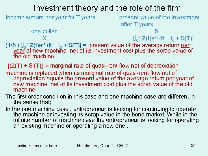Investment theory and the role of the firm Income stream per year fot T years present value of the investment after T years. one dollar δ X [∫ 0 T Z(t)e-it dt – I 0 + S(T)] (1/δ ) [∫ 0 T Z(t)e-it dt – I 0 + S(T)] = present value of the average return per year of new machine net of its investment cost plus the scrap value of the old machine. [(Z(T) + S’(T)] = marginal rate of quasi-rent flow net of depreciation machine is replaced when its marginal rate of quasi-rent flow net of depreciation equals the present value of the average return per year of new machine net of its investment cost plus the scrap value of the old machine. The first order condition in this case and one machine case are different in the sense that; In the one machine case , entrepreneur is looking for continuing to operate the machine or investing its scrap value in the bond market. While in the infinite number of machine case the entrepreneur is looking for operating an existing machine or operating a new one. optimization over time Henderson , Quandt , CH 12 35

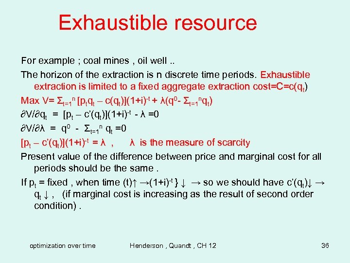Exhaustible resource For example ; coal mines , oil well. . The horizon of the extraction is n discrete time periods. Exhaustible extraction is limited to a fixed aggregate extraction cost=C=c(qt) Max V= Σt=1 n [ptqt – c(qt)](1+i)-t + λ(q 0 - Σt=1 nqt) ∂V/∂qt = [pt – c’(qt)](1+i)-t - λ =0 ∂V/∂λ = q 0 - Σt=1 n qt =0 [pt – c’(qt)](1+i)-t = λ , λ is the measure of scarcity Present value of the difference between price and marginal cost for all periods should be the same. If pt = fixed , when time (t)↑ →(1+i)-t } ↓ → so we should have c’(qt)↓ → qt ↓ , (if marginal cost is increasing as the result of second order condition). optimization over time Henderson , Quandt , CH 12 36

Human Capital Cost of education ; 1 - direct cost ; like teacher’s salaries, textbook expenditures , . . 2 - opportunity cost of earning forgone during studying ; There is three questions ; 1 - yes or no decision for continuing higher education 2 - cost of training workers 3 - optimal investment in human capital over an earning cycle Investment in education The question is whether to continue the education or enter the labor market. Two alternative income stream; 1 -graduate from high school at t 0 and enter the labor force immediately and get an income stream equal to g(t). 2 -going to college and spend t 0 to t 1 in the college. He would spend some of his income as college expenses, graduate at t 1 from college and earn an income stream equal to f(t). optimization over time Henderson , Quandt , CH 12 37

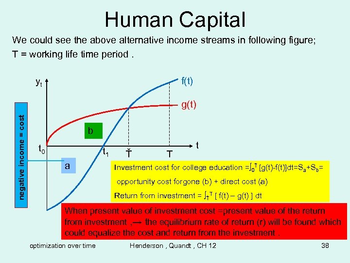Human Capital We could see the above alternative income streams in following figure; T = working life time period. yt f(t) negative income = cost g(t) b t 0 t 1 a Ť T t Investment cost for college education =∫ 0Ť [g(t)-f(t)]dt=Sa+Sb= opportunity cost forgone (b) + direct cost (a) Return from investment = ∫ŤT [ f(t) – g(t) ] dt When present value of investment cost =present value of the return from investment , → the equilibrium rate of return (r) will be found which could equalize the cost and return from the investment. optimization over time Henderson , Quandt , CH 12 38

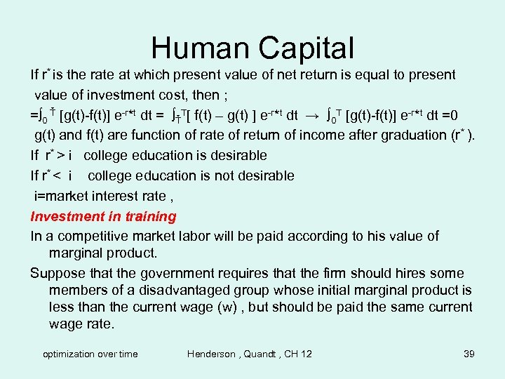Human Capital If r* is the rate at which present value of net return is equal to present value of investment cost, then ; =∫ 0 Ť [g(t)-f(t)] e-r*t dt = ∫ŤT[ f(t) – g(t) ] e-r*t dt → ∫ 0 T [g(t)-f(t)] e-r*t dt =0 g(t) and f(t) are function of rate of return of income after graduation (r* ). If r* > i college education is desirable If r* < i college education is not desirable i=market interest rate , Investment in training In a competitive market labor will be paid according to his value of marginal product. Suppose that the government requires that the firm should hires some members of a disadvantaged group whose initial marginal product is less than the current wage (w) , but should be paid the same current wage rate. optimization over time Henderson , Quandt , CH 12 39

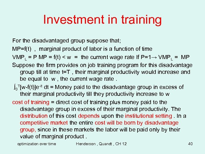Investment in training For the disadvantaged group suppose that; MP=f(t) , marginal product of labor is a function of time VMPL = P MP = f(t) < w = the current wage rate If P=1→ VMP L = MP Suppose the firm provides on job training program for this disadvantage group till at time t=T , their marginal productivity would increase and be equal to w , the current wage rate. ∫ 0 T[w-f(t)]e-it dt = Money paid to the disadvantage group in excess of their marginal productivity till they productivity increase to w cost of training = direct cost of training plus money paid to the disadvantage group in excess of their marginal productivity. The distribution of this cost depends upon the institutional setting. In a competitive market the entire cost will be born by disadvantage group, since in these markets the labor will be paid only by their value of marginal product. optimization over time Henderson , Quandt , CH 12 40

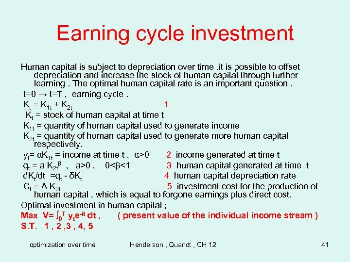Earning cycle investment Human capital is subject to depreciation over time. it is possible to offset depreciation and increase the stock of human capital through further learning. The optimal human capital rate is an important question. t=0 → t=T , earning cycle. Kt = K 1 t + K 2 t 1 Kt = stock of human capital at time t K 1 t = quantity of human capital used to generate income K 2 t = quantity of human capital used to generate more human capital respectively. yt= αK 1 t = income at time t , α>0 2 income generated at time t qt = a K 2 tβ , a>0 , 0<β<1 3 human capital generated at time t d. Kt/dt =qt - δKt 4 human capital depreciation rate Ct = A K 2 t 5 investment cost for the production of human capital , which is equal to forgone earnings plus direct cost. Optimal investment in human capital ; Max V= ∫ 0 T yte-it dt , ( present value of the individual income stream ) S. T. 1 , 2 , 3 , 4, 5 optimization over time Henderson , Quandt , CH 12 41

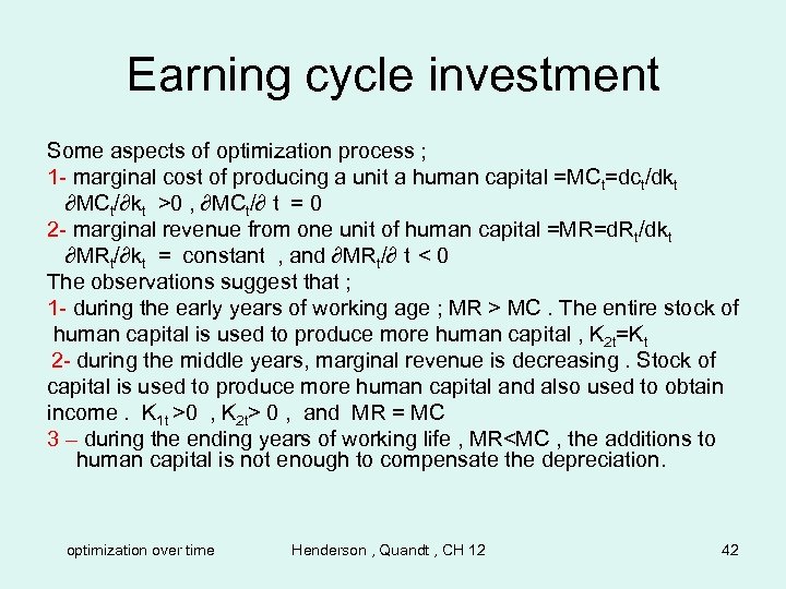Earning cycle investment Some aspects of optimization process ; 1 - marginal cost of producing a unit a human capital =MCt=dct/dkt ∂MCt/∂kt >0 , ∂MCt/∂ t = 0 2 - marginal revenue from one unit of human capital =MR=d. Rt/dkt ∂MRt/∂kt = constant , and ∂MRt/∂ t < 0 The observations suggest that ; 1 - during the early years of working age ; MR > MC. The entire stock of human capital is used to produce more human capital , K 2 t=Kt 2 - during the middle years, marginal revenue is decreasing. Stock of capital is used to produce more human capital and also used to obtain income. K 1 t >0 , K 2 t> 0 , and MR = MC 3 – during the ending years of working life , MR

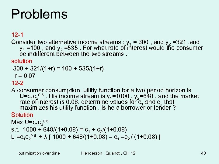Problems 12 -1 Consider two alternative income streams ; y 1 = 300 , and y 2 =321 , and y 1 =100 , and y 2 =535. For what rate of interest would the consumer be indifferent between the two streams. solution 300 + 321/(1+r) = 100 + 535/(1+r) r = 0. 07 12 -2 A consumer consumption–utility function for a two period horizon is U=c 1 c 20. 6. His income stream is y 1=1000 , y 2=648 , and the market rate of interest is 0. 08. determine values for c 1 and c 2 that maximizes his utility function. Is he a borrower or lender ? Solution Max U=c 1 c 20. 6 s. t. 1000 + 648/(1+0. 08) = c 1 + c 2/(1+0. 08) L =c 1 c 20. 6 + λ [ 1000 + 648/(1+0. 08) – c 1 –c 2 / (1+0. 08) ] optimization over time Henderson , Quandt , CH 12 43

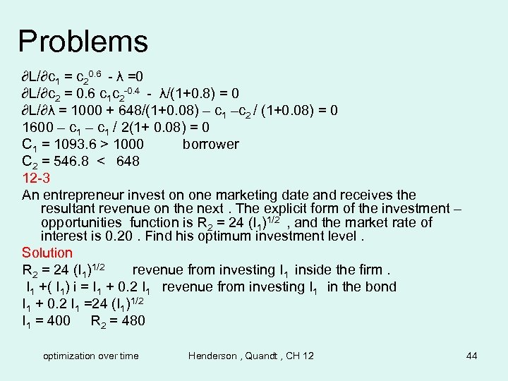Problems ∂L/∂c 1 = c 20. 6 - λ =0 ∂L/∂c 2 = 0. 6 c 1 c 2 -0. 4 - λ/(1+0. 8) = 0 ∂L/∂λ = 1000 + 648/(1+0. 08) – c 1 –c 2 / (1+0. 08) = 0 1600 – c 1 / 2(1+ 0. 08) = 0 C 1 = 1093. 6 > 1000 borrower C 2 = 546. 8 < 648 12 -3 An entrepreneur invest on one marketing date and receives the resultant revenue on the next. The explicit form of the investment – opportunities function is R 2 = 24 (I 1)1/2 , and the market rate of interest is 0. 20. Find his optimum investment level. Solution R 2 = 24 (I 1)1/2 revenue from investing I 1 inside the firm. I 1 +( I 1) i = I 1 + 0. 2 I 1 revenue from investing I 1 in the bond I 1 + 0. 2 I 1 =24 (I 1)1/2 I 1 = 400 R 2 = 480 optimization over time Henderson , Quandt , CH 12 44

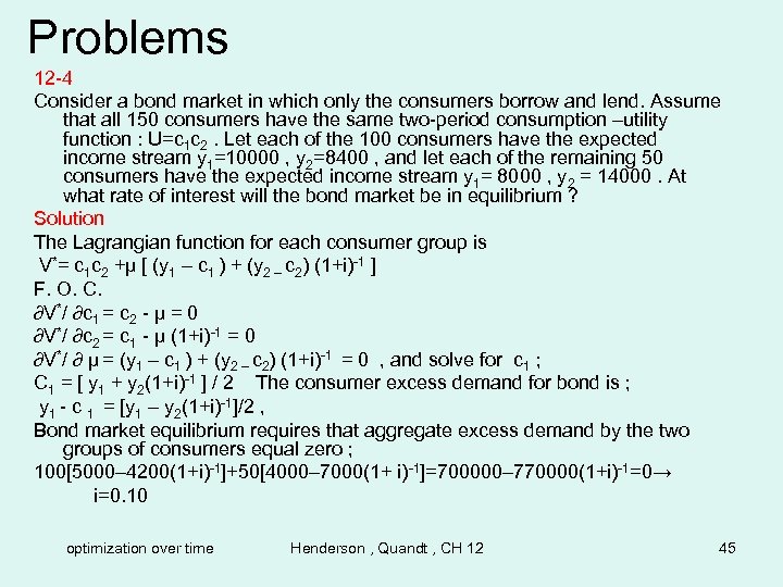Problems 12 -4 Consider a bond market in which only the consumers borrow and lend. Assume that all 150 consumers have the same two-period consumption –utility function : U=c 1 c 2. Let each of the 100 consumers have the expected income stream y 1=10000 , y 2=8400 , and let each of the remaining 50 consumers have the expected income stream y 1= 8000 , y 2 = 14000. At what rate of interest will the bond market be in equilibrium ? Solution The Lagrangian function for each consumer group is V*= c 1 c 2 +µ [ (y 1 – c 1 ) + (y 2 – c 2) (1+i)-1 ] F. O. C. ∂V*/ ∂c 1 = c 2 - µ = 0 ∂V*/ ∂c 2 = c 1 - µ (1+i)-1 = 0 ∂V*/ ∂ µ = (y 1 – c 1 ) + (y 2 – c 2) (1+i)-1 = 0 , and solve for c 1 ; C 1 = [ y 1 + y 2(1+i)-1 ] / 2 The consumer excess demand for bond is ; y 1 - c 1 = [y 1 – y 2(1+i)-1]/2 , Bond market equilibrium requires that aggregate excess demand by the two groups of consumers equal zero ; 100[5000– 4200(1+i)-1]+50[4000– 7000(1+ i)-1]=700000– 770000(1+i)-1=0→ i=0. 10 optimization over time Henderson , Quandt , CH 12 45

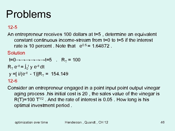Problems 12 -5 An entrepreneur receives 100 dollars at t=5 , determine an equivalent constant continuous income-stream from t=0 to t=5 if the interest rate is 10 percent. Note that e 0. 5 = 1. 64872. Solution t=0→→→→→→t=5. RT = 100 RT e-it = ∫ 0 t y e-it dt y =[ i/(e-it - 1)]RT = 154. 149 12 -6 Consider an entrepreneur engaged in a point input point output vinegar aging process. his initial cost is 20 , the sales value of the vinegar is R(T)=100 T 1/2. And the rate of interest is 0. 05. How long is his optimal investment period. optimization over time Henderson , Quandt , CH 12 46

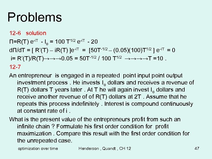Problems 12 -6 solution Π=R(T) e-i. T - Io = 100 T 1/2 e-i. T - 20 dΠ/d. T = [ R’(T) – i. R(T) ]e-i. T = [50 T-1/2 – (0. 05)(100)T 1/2 ] e-i. T = 0 i= R’(T)/R(T)→→→ 0. 05 = 50 T-1/2 / 100 T 1/2 →→→→T =10. 12 -7 An entrepreneur is engaged in a repeated point input point output investment process. He invests Io dollars and receives a revenue of R(T) dollars T years later. At T he will again invest Io dollars and receive another revenue of of R(T) dollars at 2 T. Assume that he repeats this process indefinitely. Interest is compound continuously at constant rate of i. What is the present value of the entrepreneurs profit from such an infinite chain ? Formulate his first order condition for profit maximization. Compare this result with the first order condition for the unrepeated case. optimization over time Henderson , Quandt , CH 12 47

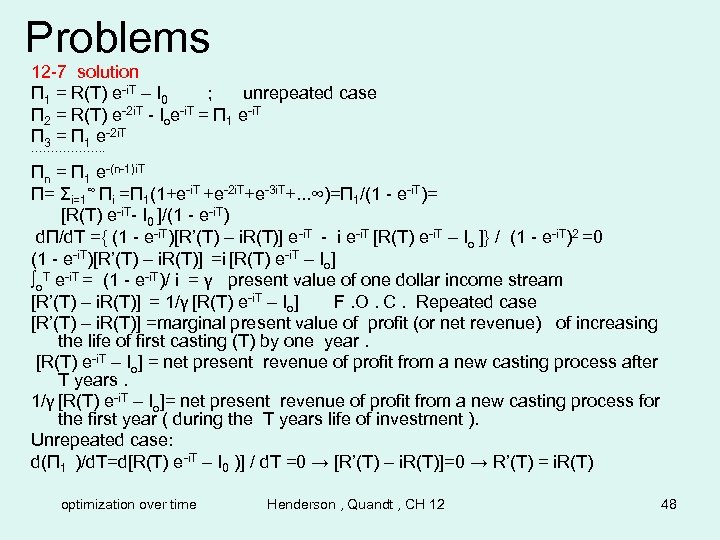Problems 12 -7 solution Π 1 = R(T) e-i. T – I 0 ; unrepeated case Π 2 = R(T) e-2 i. T - Ioe-i. T = Π 1 e-i. T Π 3 = Π 1 e-2 i. T ………………. Πn = Π 1 e-(n-1)i. T Π= Σi=1∞ Πi =Π 1(1+e-i. T +e-2 i. T+e-3 i. T+. . . ∞)=Π 1/(1 - e-i. T)= [R(T) e-i. T- I 0 ]/(1 - e-i. T) dΠ/d. T ={ (1 - e-i. T)[R’(T) – i. R(T)] e-i. T - i e-i. T [R(T) e-i. T – Io ]} / (1 - e-i. T)2 =0 (1 - e-i. T)[R’(T) – i. R(T)] =i [R(T) e-i. T – Io] ∫o. T e-i. T = (1 - e-i. T)/ i = γ present value of one dollar income stream [R’(T) – i. R(T)] = 1/γ [R(T) e-i. T – Io] F. O. C. Repeated case [R’(T) – i. R(T)] =marginal present value of profit (or net revenue) of increasing the life of first casting (T) by one year. [R(T) e-i. T – Io] = net present revenue of profit from a new casting process after T years. 1/γ [R(T) e-i. T – Io]= net present revenue of profit from a new casting process for the first year ( during the T years life of investment ). Unrepeated case: d(Π 1 )/d. T=d[R(T) e-i. T – I 0 )] / d. T =0 → [R’(T) – i. R(T)]=0 → R’(T) = i. R(T) optimization over time Henderson , Quandt , CH 12 48

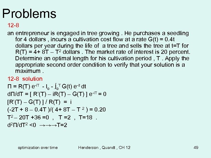Problems 12 -8 an entrepreneur is engaged in tree growing. He purchases a seedling for 4 dollars , incurs a cultivation cost flow at a rate G(t) = 0. 4 t dollars per year during the life of a tree and sells the tree at t=T for R(T) = 4+ 8 T – T 2 dollars. The market rate of interest is 20 percent. Determine an optimal length for his cultivation period , T. Apply the appropriate second order condition to verify that your solution is a maximum. 12 -8 solution Π = R(T) e-i. T - Io - ∫o. T G(t) e-it dt dΠ/d. T = [ R’(T) – i. R(T) – G(T) ] e-i. T = 0 [R’(T) – G(T) ] / R(T) = i (-2 T + 8 – 0. 4 T )/( 4+ 8 T – T 2 ) = 0. 20 T 2 – 20 T +36 =0 , T =2 , T=18. d 2Π/d. T 2 <0 →→→T=2 optimization over time Henderson , Quandt , CH 12 49

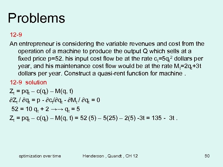Problems 12 -9 An entrepreneur is considering the variable revenues and cost from the operation of a machine to produce the output Q which sells at a fixed price p=52. his input cost flow be at the rate ct=5 qt 2 dollars per year, and his maintenance cost flow would be at the rate Mt=2 qt+3 t dollars per year. Construct a quasi-rent function for machine. 12 -9 solution Zt = pqt – c(qt) – M(q, t) ∂Zt / ∂qt = p - ∂ct/∂qt - ∂Mt / ∂qt = 0 52 = 10 qt + 2 →→ qt = 5 Zt = pqt – c(qt) – M(q, t) = 52 (5) – 5(25) – 2(5) -3 t = 135 - 3 t. optimization over time Henderson , Quandt , CH 12 50

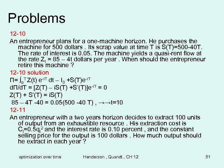Problems 12 -10 An entrepreneur plans for a one-machine horizon. He purchases the machine for 500 dollars. Its scrap value at time T is S(T)=500 -40 T. The rate of interest is 0. 05. The machine yields a quasi-rent flow at the rate Zt = 85 – 4 t dollars per year. When should the entrepreneur retire this machine ? 12 -10 solution Π= ∫o. T Z(t) e-i. T dt – I 0 +S(T)e-i. T dΠ/d. T = [Z(T) – i. S(T) +S’(T)]e-i. T = 0 Z(T) + S’(T) = i. S(T) 85 – 4 T -40 = 0. 05(500 -40 T) , →→t=10 12 -11 An entrepreneur with a two years horizon decides to extract 100 units of output from an exhaustible resource. His extraction cost is Ct=0. 5 qt 2 and the interest rate is 0. 10 percent , and the constant selling price for the output is 100 dollars. How much output should he extract in each year ? optimization over time Henderson , Quandt , CH 12 51

Problems 12 -11 solution Max Π= Σt=1 t=2 [ ptqt – c(qt) ] (1+i)-t + λ(q 0 – Σt=1 t=2 qt) dΠ/dqt = 0 →→→ [Pt - c’(qt) ] (1+i)-t = λ [P 1 - c’(q 1 ) ] (1+i)-1 = λ [P 2 - c’(q 2 ) ] (1+i)-2 = λ [P 1 - c’(q 1 ) ] = [P 2 - c’(q 2 ) ] (1+i)-1 (100 –q 1) = (100 – q 2)(1. 01)-1 q 1+q 2=100 q 1 = 52. 3 q 2 = 47. 7 THE END optimization over time Henderson , Quandt , CH 12 52

optimization over time Henderson , Quandt , CH 12 53