Intro to R Programming Lecture 1 Evan Girvetz

Intro to R Programming: Lecture 1 Evan Girvetz girvetz@u. washington. edu 206 -543 -5772 © R Foundation, from http: //www. r-project. org 209 Winkenwerder

What is R? • R is a language and environment for statistical computing and graphics • The term "environment" is intended to characterize it as a fully planned and coherent system, rather than an incremental accretion of very specific and inflexible tools, as is frequently the case with other data analysis software.

What is R? • It is a open source computer programming project which is similar to the S language and environment, which was developed at Bell Laboratories (formerly AT&T, now Lucent Technologies) by John Chambers and colleagues. • R can be considered as a different implementation of S.

What is R? • an effective data handling and storage facility • a suite of operators for calculations on arrays and matrices • a large, coherent, integrated collection of tools for data analysis • graphical facilities for data analysis and display either onscreen or on hardcopy • a well-developed, simple and effective programming language which includes conditionals, loops, userdefined recursive functions and input and output facilities.

Where to get R • The R-project web site: – http: //www. r-project. org • The program can be downloaded from any one of the official mirrors of CRAN – http: //cran. r-project. org – Download the compiled binary code for your operating system – See supplemental material on website describing how to download and install R

What can R do? • R provides a comprehensive set of statistical analysis techniques – Classical statistical tests – Linear and nonlinear modeling – Time-series analysis – Classification & cluster analysis – Spatial statistics – Basically any statistical technique you can think of is part of a contributed package to R

What can R do? • Contributed Packages are a feature of R that allows it to be a very powerful data analysis and graphing environment • The community of users contributes these packages. – 1689 Contributed Packages – New packages are continuously being added

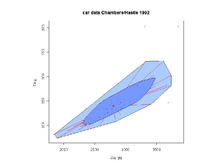
What can R do? • Publication-quality plots can be produced – Many default graphing choices – The user retains full control of the graphics – Including mathematical symbols and formulae

R is a Language • R is a language that you can learn to communicate to the computer what you would like it to do • Just like with other languages, the initial learning curve can be steep, but there are dictionaries and other resources for assistance – help(function) – ? function • The benefits of becoming fluent can be very rewarding

Using R: Hands-on Introduction Prompt

R Reference Material • Intro to R (PDF available from help menu) • Many books to reference – Data Analysis and Graphics Using R, 2 nd ed. (Maindonald & Braun) – The R Book (Michael Crawley) – Modern Applied Statistics with S-plus • R Ref card (Tom Short)

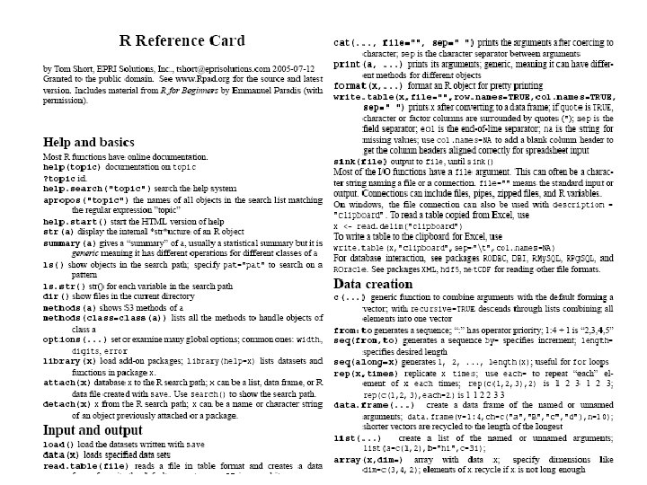
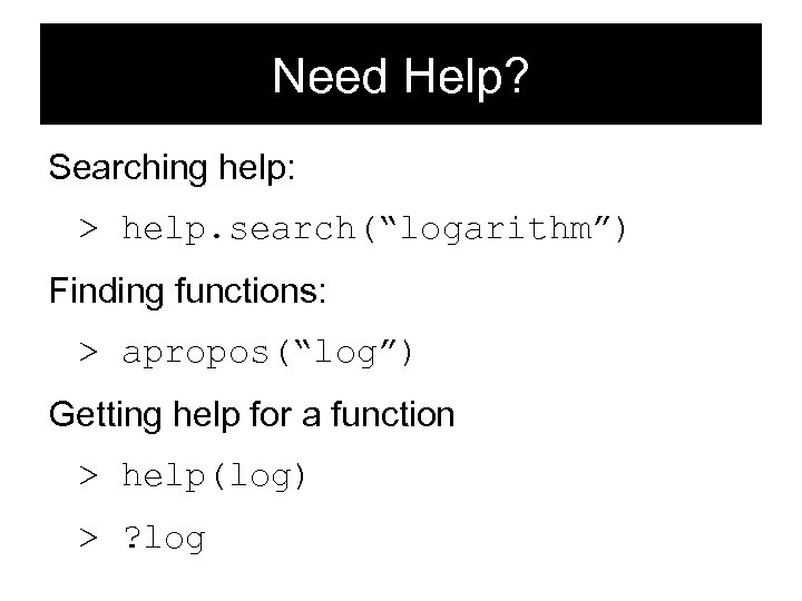Need Help? Searching help: > help. search(“logarithm”) Finding functions: > apropos(“log”) Getting help for a function > help(log) > ? log

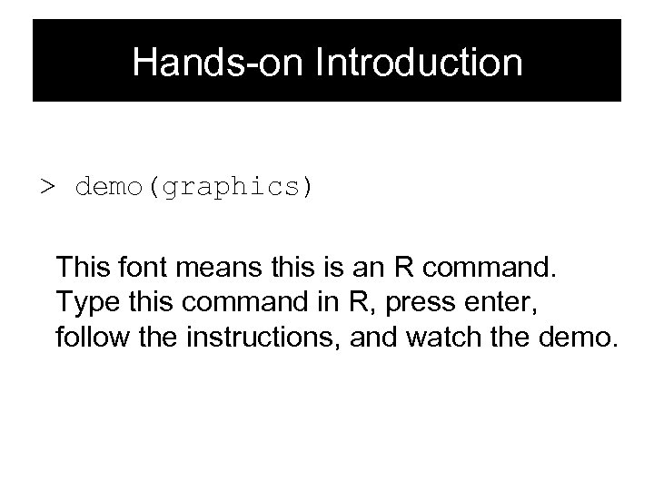Hands-on Introduction > demo(graphics) This font means this is an R command. Type this command in R, press enter, follow the instructions, and watch the demo.

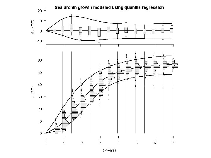
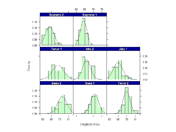
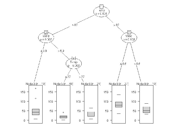
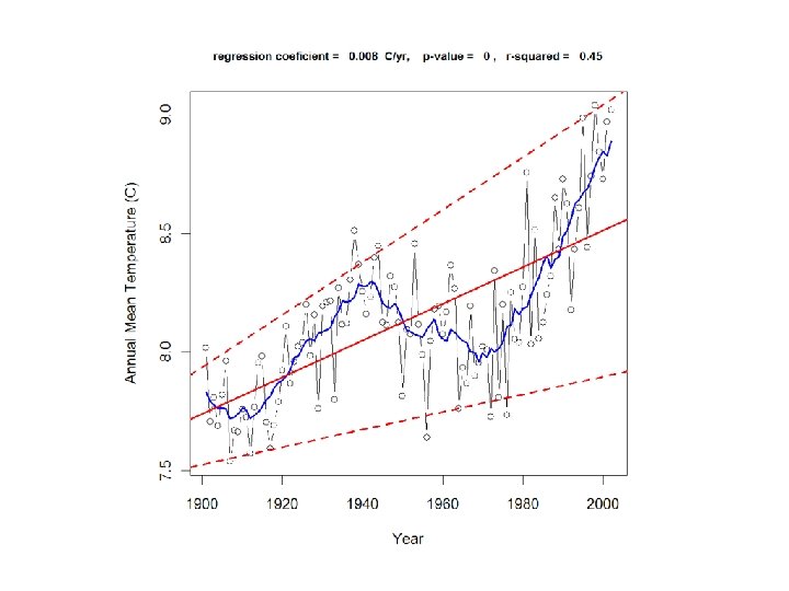
Examples of Graphics Created Using R

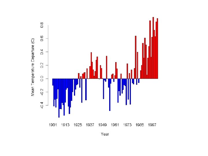
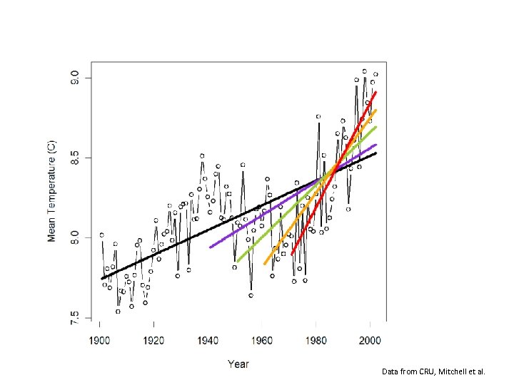Data from CRU, Mitchell et al.

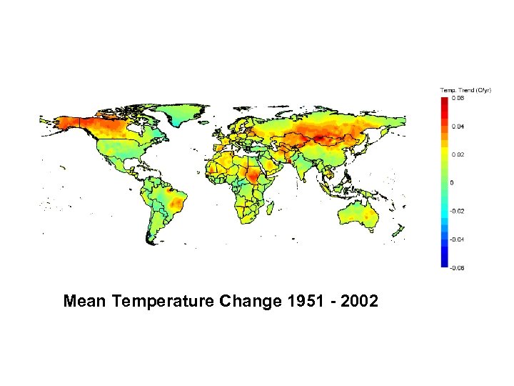Climate Does Not Change the Same Everywhere Mean Temperature Change 1951 - 2002

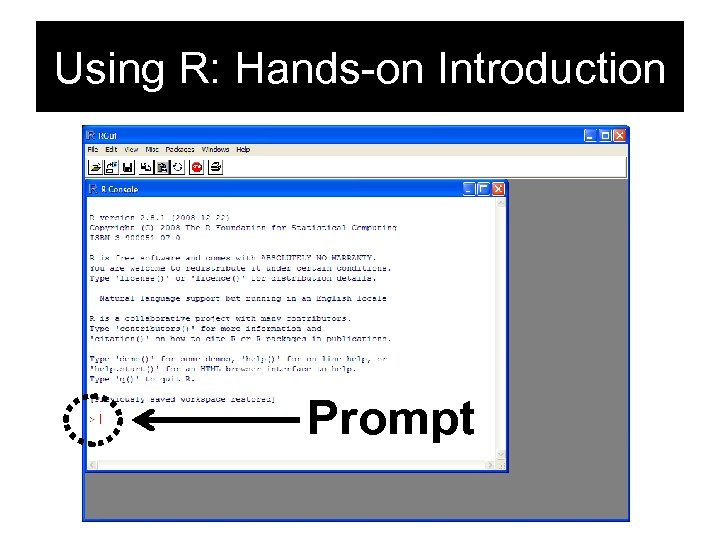Using R: Hands-on Introduction Prompt

R workspaces • All analyses are saved in an R workspace • The location of the workspace should be specified at the beginning of an R session • You can save R workspaces (. Rdata)

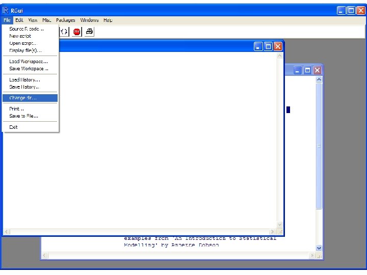
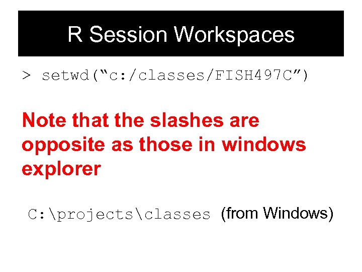R Session Workspaces > setwd(“c: /classes/FISH 497 C”) Note that the slashes are opposite as those in windows explorer C: projectsclasses (from Windows)

Using R: Hands-on Introduction Prompt

Some Simple R Commands > 2+2 Result [1] 4 > log(42) Function Argument(s) inside parentheses

Some Simple R Commands > log(42) [1] 3. 737670 Command Result Log base e natural logarithm ln(x)

Some Simple R Commands > log(42, base = 10) [1] 1. 623249 Log base 10 Result

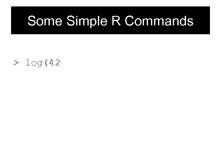Some Simple R Commands > log(42

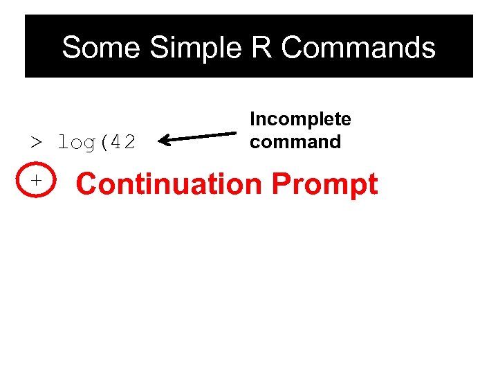Some Simple R Commands > log(42 + Incomplete command Continuation Prompt

Some Simple R Commands > log(42 + , base = 10) [1] 1. 623249 Continuation

Object Oriented Language • R is an object oriented language • Essentially everything in R is an object – Number – Data table – Function (e. g. ANOVA analysis) – Model output (e. g. ANOVA output object) – Graph – Etc.

Object Oriented Language • Objects are stored in the directory you have told R to work in – the output from a computation (e. g. log(42)) or analysis (e. g. ANOVA) can be stored as an object to be viewed later, or used in a later analysis

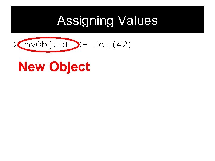Assigning Values > my. Object <- log(42) New Object

Assigning Values > my. Object <- log(42) > my. Object [1] 3. 737670 my. Object is an object that contains the calculation result

Assigning Values > my. Object * 10 [1] 37. 37670 Multiply my. Object by 10

rm(my. Object) Remove objects" src="https://present5.com/presentation/4891d4324dce4e78c1e4a7d99f29e174/image-42.jpg" alt="Managing Objects > ls() List objects [1] "my. Object" > rm(my. Object) Remove objects" /> Managing Objects > ls() List objects [1] "my. Object" > rm(my. Object) Remove objects

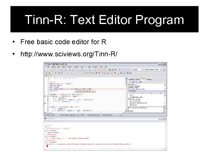Tinn-R: Text Editor Program • Free basic code editor for R • http: //www. sciviews. org/Tinn-R/

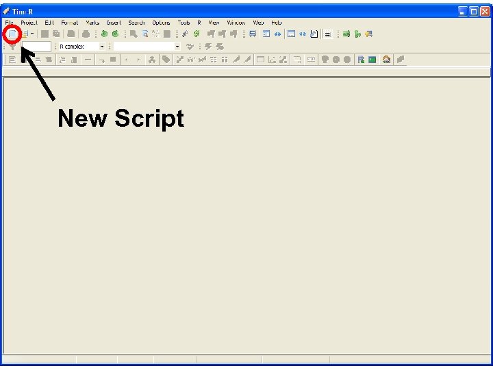New Script

Save Your Scripts!!! 1. Save your Scripts 2. Save your Scripts 3. Save your Scripts Save your scripts so you can re-run your analyses later and use them to build upon for other scripts

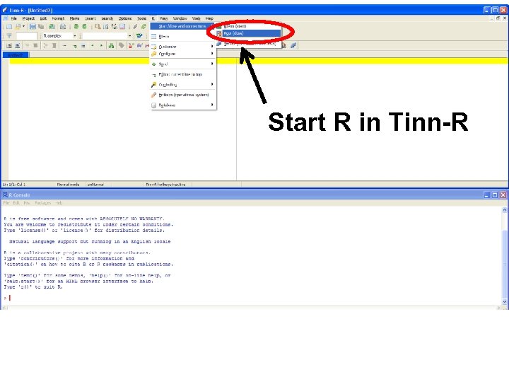Start R in Tinn-R

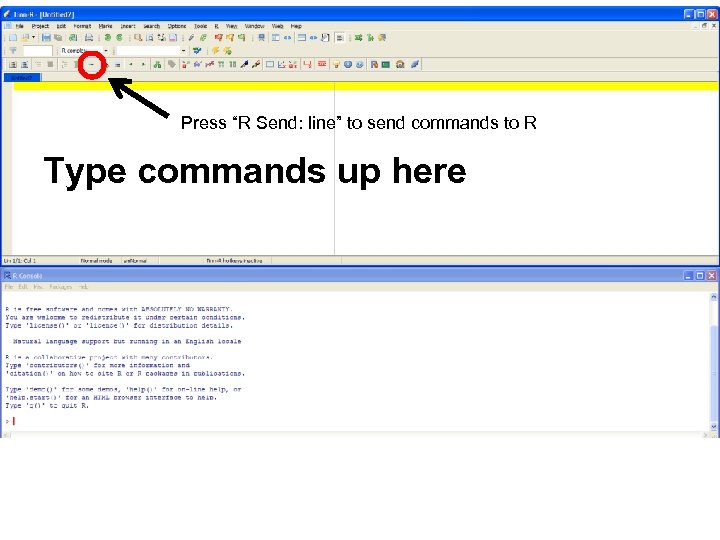Press “R Send: line” to send commands to R Type commands up here

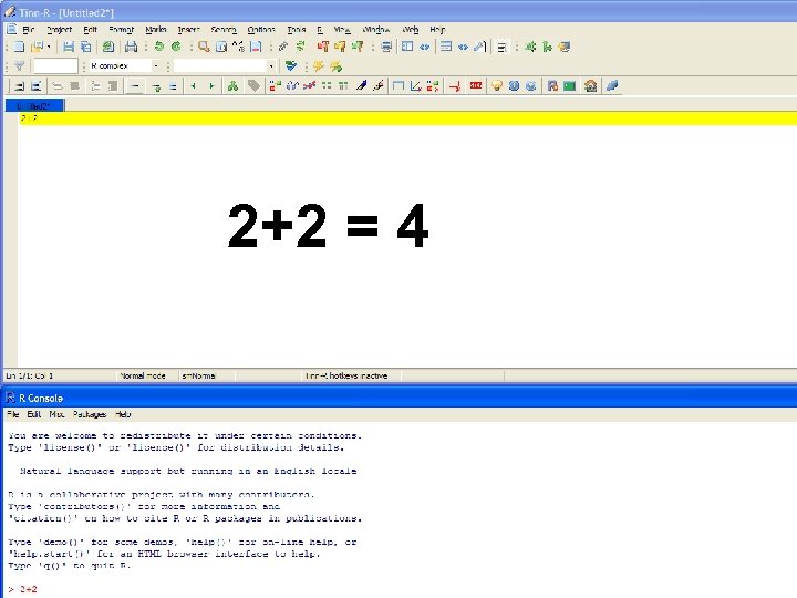2+2 = 4

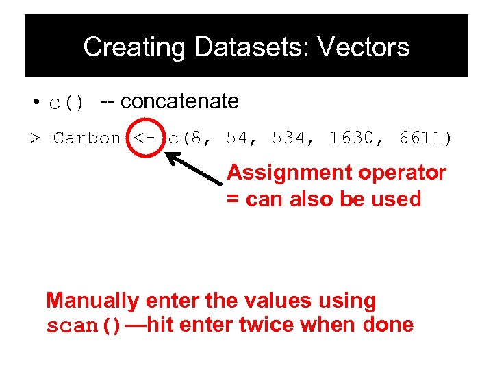Creating Datasets: Vectors • c() -- concatenate > Carbon <- c(8, 54, 534, 1630, 6611) > Carbon [1] 1 Assignment operator 5 14 15= can 8 6 also be used > Carbon <- scan() Manually enter the values using scan()—hit enter twice when done

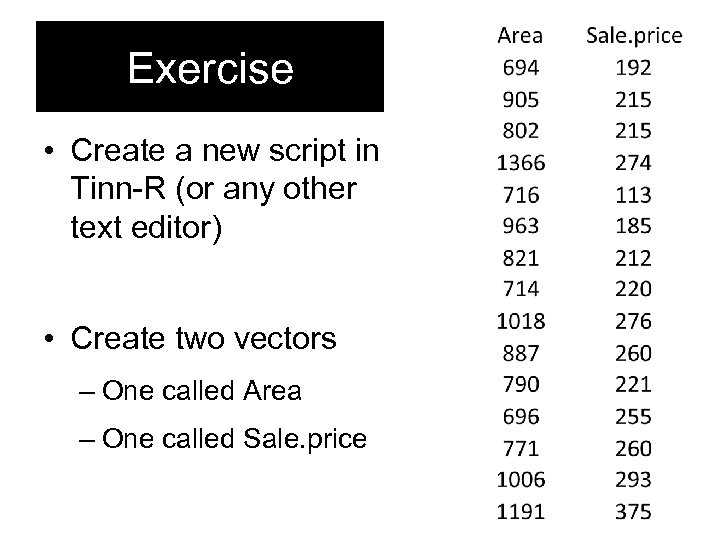Exercise • Create a new script in Tinn-R (or any other text editor) • Create two vectors – One called Area – One called Sale. price

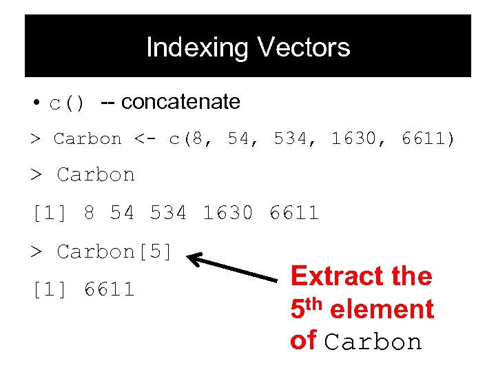Indexing Vectors • c() -- concatenate > Carbon <- c(8, 54, 534, 1630, 6611) > Carbon [1] 8 54 534 1630 6611 > Carbon[5] [1] 6611 Extract the 5 th element of Carbon

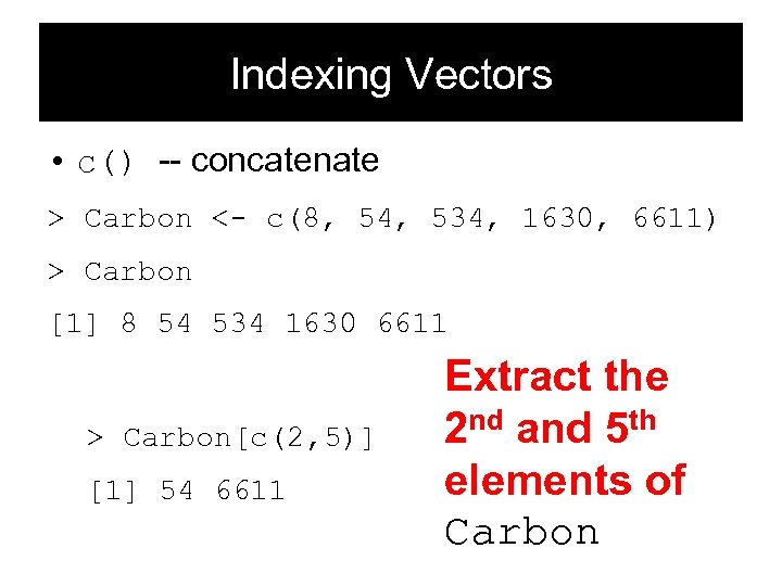Indexing Vectors • c() -- concatenate > Carbon <- c(8, 54, 534, 1630, 6611) > Carbon [1] 8 54 534 1630 6611 > Carbon[c(2, 5)] [1] 54 6611 Extract the 2 nd and 5 th elements of Carbon

Indexing Vectors > Carbon [1] 8 54 534 1630 6611 > Carbon[c(3, 4)] [1] 534 1630 > Carbon[-c(3, 4)] [1] 8 54 6611 3 rd and 4 th elements of vector only All elements except for the 3 rd and 4 th

Indexing Vectors > Carbon [1] 8 54 534 1630 6611 > Carbon[2: 4] [1] 54 534 1630 > Carbon[-(2: 4)] [1] 8 6611 2 ne through 4 th elements of vector only All elements except for the 2 nd through 4 th

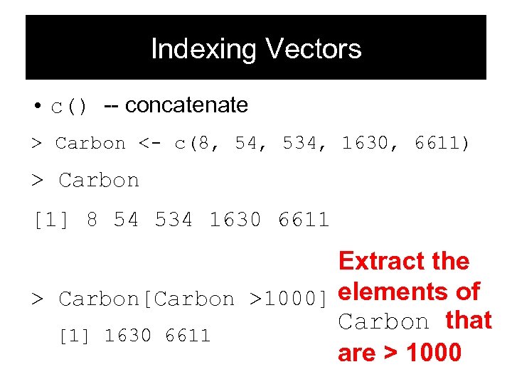Indexing Vectors • c() -- concatenate > Carbon <- c(8, 54, 534, 1630, 6611) > Carbon [1] 8 54 534 1630 6611 Extract the > Carbon[Carbon >1000] elements of Carbon that [1] 1630 6611 are > 1000

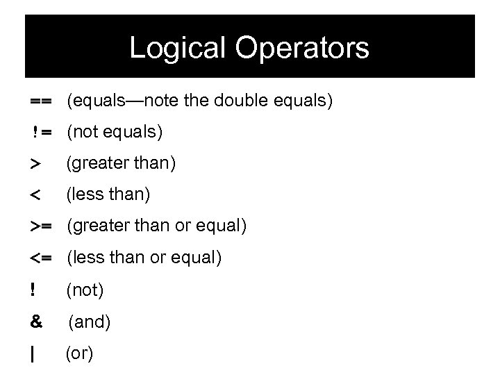Logical Operators == (equals—note the double equals) != (not equals) > (greater than) < (less than) >= (greater than or equal) <= (less than or equal) ! (not) & (and) | (or)

Logical Operators > Carbon>1000 [1] FALSE Greater Than FALSE TRUE Logical Operators return TRUE or FALSE > c(FALSE, TRUE)

Indexing Vectors > Carbon[c(F, F, F, T, T)] [1] 1630 6611 Elements can be extracted using TRUE & False— must use c()

Logical Operators > Carbon [1] 8 54 534 1630 6611 > Carbon>1000 [1] FALSE TRUE > Carbon<5000 [1] TRUE FALSE

Logical Operators > Carbon [1] 8 54 534 1630 6611 > bool <- (Carbon>1000)|(Carbon<5000) [1] FALSE TRUE FALSE > Carbon[bool] [1] 1630 Note difference between [] and ()

Difference between [] and () > Carbon[(Carbon>1000)|(Carbon<5000)] [1] 1630 [] – square brackets are used for indexing objects--pulling out different values () – round brackets or parentheses are used for functions and operators

Hands-on Exercise Create and object called Year: > Year [1] 1800 1850 1900 1950 2000

Indexing Vectors > Carbon [1] 8 54 534 1630 6611 > Year [1] 1800 1850 1900 1950 2000 > Carbon[Year>=1900] Index a vector based on values [1] 534 1630 6611 of another vector Both vectors must be the same size

Summary of Extracting Data Based on logical values > Carbon[Year>=1900] [1] 534 1630 6611 Based on numerical indicies > Carbon[c(3, 4)]

Hands-On Exercise • Using the Sale. price and Area vectors you produced earlier, produce a vector called Sale. price. gt 1000 that contains only sale prices for houses with an area greater than 1000. • Similarly, create a vector called Area. gt 1000 that only contains the areas greater than 1000

Patterned Data: seq() Sequence > 1: 5 [1] 1 2 3 4 5 > seq(from = 1, to = 5, by=1) [1] 1 2 3 4 5 > seq(from = 1800, to = 2000, by=50) [1] 1800 1850 1900 1950 2000

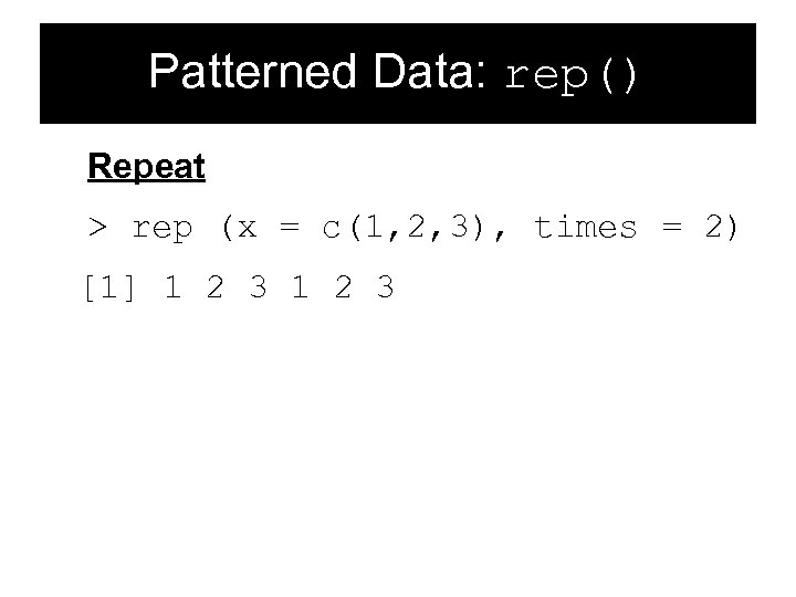Patterned Data: rep() Repeat > rep (x = c(1, 2, 3), times = 2) [1] 1 2 3

Dimension of data > new. Data <- 1: 20 [1] 1 2 3 4 5 6 7 8 9 [10] 10 11 12 13 14 15 16 17 18 [19] 19 20 > matrix(new. Data, 5, 4 byrow = T) [, 1] [, 2] [, 3] [, 4] [1, ] 1 6 11 16 [2, ] 2 7 12 17 [3, ] 3 8 13 18 [4, ] 4 9 14 19 [5, ] 5 10 15 20 Five rows by four columns

Dimension of data > new. Data <- 1: 20 [1] 1 2 3 4 5 6 7 8 9 [10] 10 11 12 13 14 15 16 17 18 [19] 19 20 > dim(new. Data) <- c(5, 4) [, 1] [, 2] [, 3] [, 4] [1, ] 1 6 11 16 [2, ] 2 7 12 17 [3, ] 3 8 13 18 [4, ] 4 9 14 19 [5, ] 5 10 15 20 Five rows by four columns

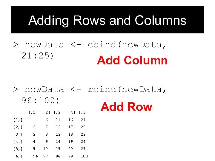Adding Rows and Columns > new. Data <- cbind(new. Data, 21: 25) Add Column > new. Data <- rbind(new. Data, 96: 100) [, 1] [, 2] [, 3] [, 4] [, 5] [1, ] 1 6 11 16 21 [2, ] 2 7 12 17 22 [3, ] 3 8 13 18 23 [4, ] 4 9 14 19 24 [5, ] 5 10 15 20 25 [6, ] 96 97 98 99 100 Add Row

Length and Dimension > dim(new. Data) [1] 6 5 > length(new. Data) [1] 30

Hands-On Exercise • Create a vector called ID. sale that gives can be used to give each house sale a unique ID number ordered starting from 1 – Hint: use length() command

Indexing Matrices > new. Data[2: 4, 1: 2] [, 1] [, 2] [1, ] 2 7 [2, ] 3 8 [3, ] 4 [rows, columns] 9 > new. Data[c(1, 3, 5), c(1: 2)] [, 1] [, 2] [1, ] 1 6 [2, ] 3 8 [3, ] 5 10 Memorize [rows, cols] (it will make your life much easier)

Data Frames • All elements of any column must be of the same type • Analogous to an Excel spread sheet

Data Frames • In general, it is best to import data frames from text files that were prepared and created in a spreadsheet program (e. g. Excel) – We will learn how to do this • However, I first want you to learn how to make a data frame from scratch in R

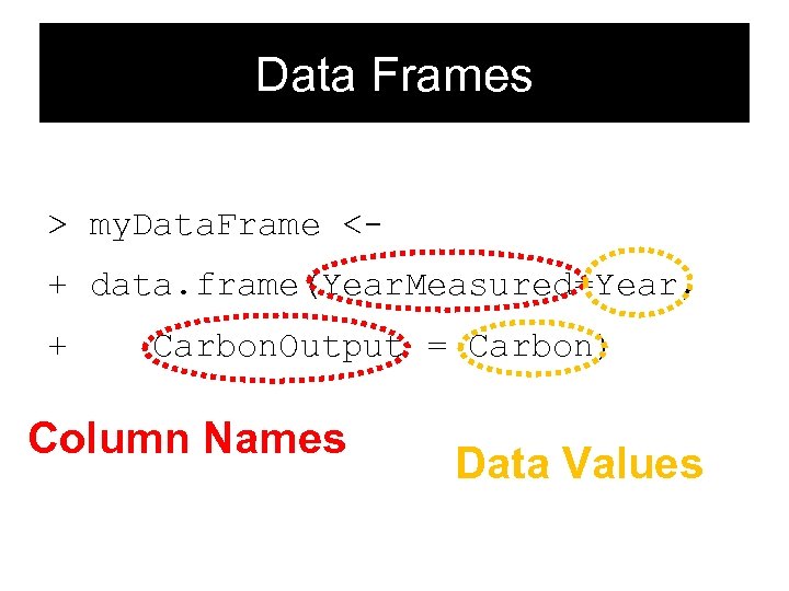Data Frames > my. Data. Frame <+ data. frame(Year. Measured=Year, + Carbon. Output = Carbon) Column Names Data Values

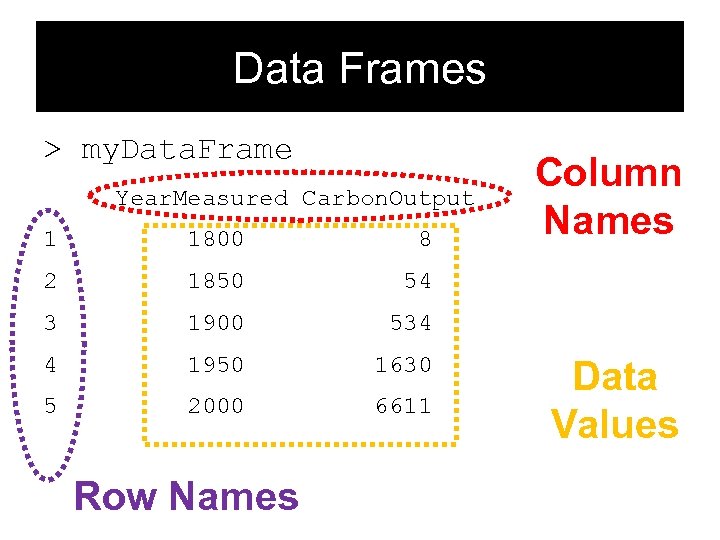Data Frames > my. Data. Frame Year. Measured Carbon. Output 1 1800 8 2 1850 54 3 1900 534 4 1950 1630 5 2000 6611 Column Names Row Names Data Values

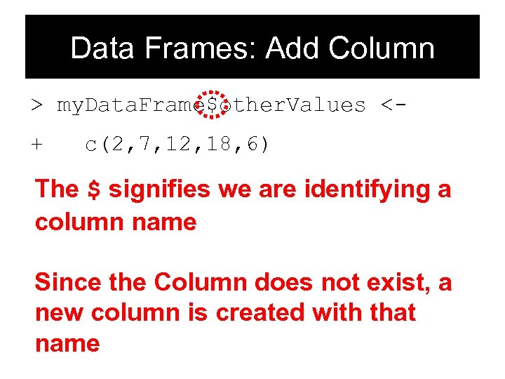Data Frames: Add Column > my. Data. Frame$other. Values <+ c(2, 7, 12, 18, 6) The $ signifies we are identifying a column name Since the Column does not exist, a new column is created with that name

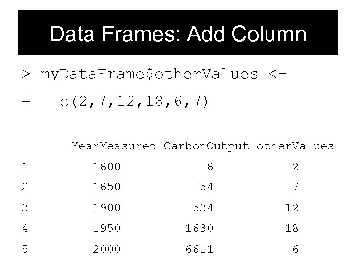Data Frames: Add Column > my. Data. Frame$other. Values <+ c(2, 7, 12, 18, 6, 7) Year. Measured Carbon. Output other. Values 1 1800 8 2 2 1850 54 7 3 1900 534 12 4 1950 1630 18 5 2000 6611 6

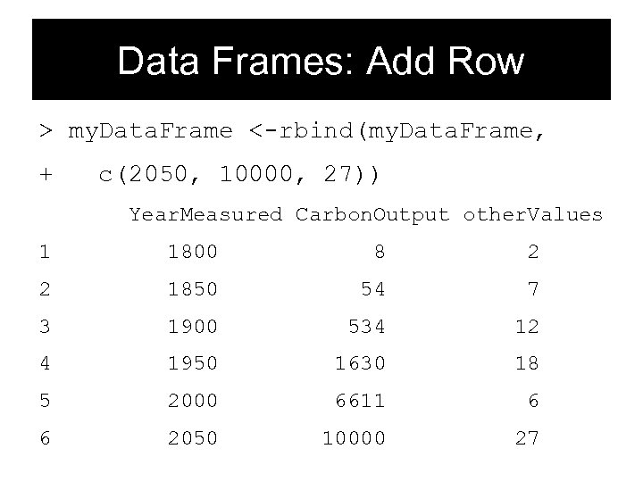Data Frames: Add Row > my. Data. Frame <-rbind(my. Data. Frame, + c(2050, 10000, 27)) Year. Measured Carbon. Output other. Values 1 1800 8 2 2 1850 54 7 3 1900 534 12 4 1950 1630 18 5 2000 6611 6 6 2050 10000 27

Remove Row > my. Data. Frame <+ my. Data. Frame[-6, ] Keep all except the 6 th row

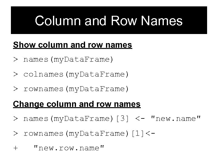Column and Row Names Show column and row names > names(my. Data. Frame) > colnames(my. Data. Frame) > rownames(my. Data. Frame) Change column and row names > names(my. Data. Frame)[3] <- "new. name" > rownames(my. Data. Frame)[1]<+ "new. row. name"

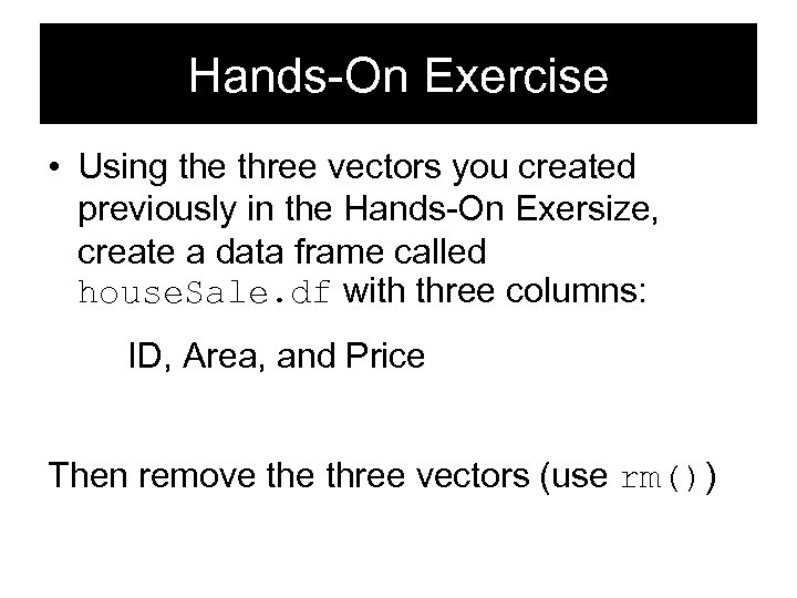Hands-On Exercise • Using the three vectors you created previously in the Hands-On Exersize, create a data frame called house. Sale. df with three columns: ID, Area, and Price Then remove three vectors (use rm())

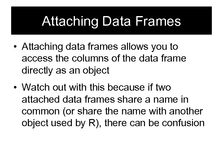Attaching Data Frames • Attaching data frames allows you to access the columns of the data frame directly as an object • Watch out with this because if two attached data frames share a name in common (or share the name with another object used by R), there can be confusion

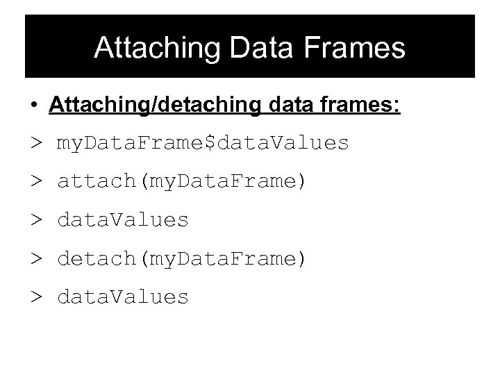Attaching Data Frames • Attaching/detaching data frames: > my. Data. Frame$data. Values > attach(my. Data. Frame) > data. Values > detach(my. Data. Frame) > data. Values

Indexing Data Frames Index frames using [rows, columns]: > my. Data. Frame[1, 2] Blank index > my. Data. Frame[1: 3, 1: 2] means all values (rows or > my. Data. Frame[, 1: 2] columns) > my. Data. Frame[, c(“Year. Measured”, “Carbon. Output")] > my. Data. Frame[, -c(2, 3)]

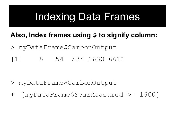Indexing Data Frames Also, Index frames using $ to signify column: > my. Data. Frame$Carbon. Output [1] 8 54 534 1630 6611 > my. Data. Frame$Carbon. Output + [my. Data. Frame$Year. Measured >= 1900]

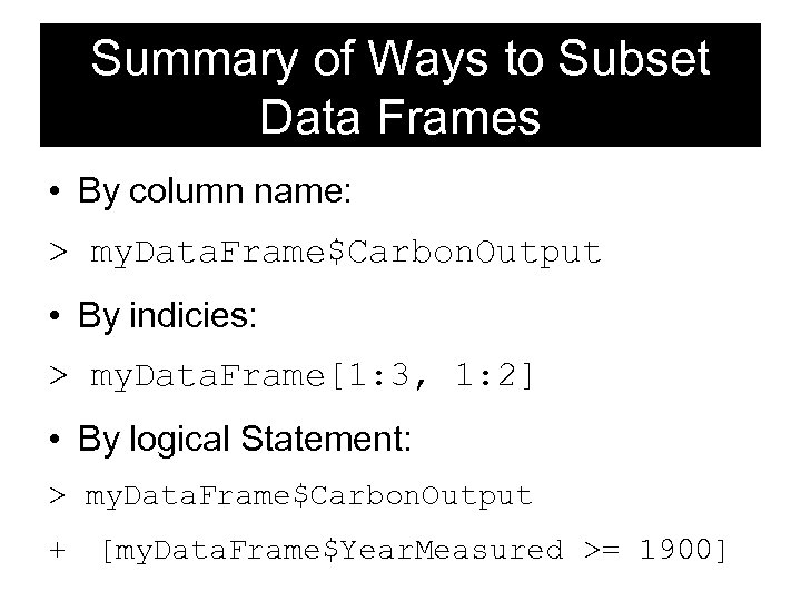Summary of Ways to Subset Data Frames • By column name: > my. Data. Frame$Carbon. Output • By indicies: > my. Data. Frame[1: 3, 1: 2] • By logical Statement: > my. Data. Frame$Carbon. Output + [my. Data. Frame$Year. Measured >= 1900]

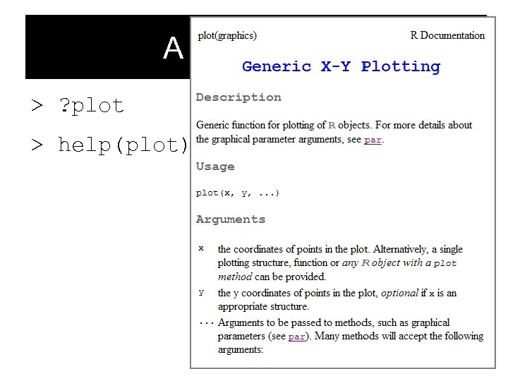A Simple Plot > ? plot > help(plot)

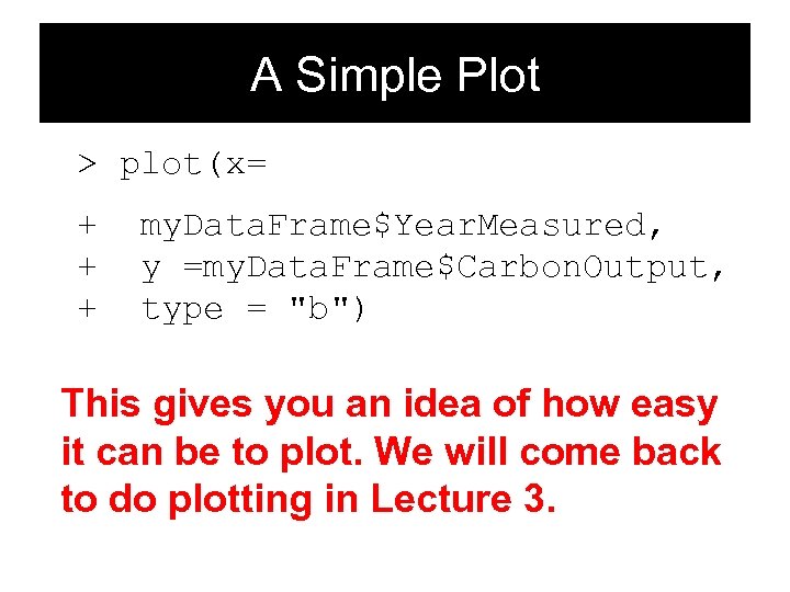A Simple Plot > plot(x= + + + my. Data. Frame$Year. Measured, y =my. Data. Frame$Carbon. Output, type = "b") This gives you an idea of how easy it can be to plot. We will come back to do plotting in Lecture 3.

Hands-On Exercise 1. Plot Sale. price versus Area 2. Use the hist() command to plot a histogram of the sale prices 3. Repeat 1 & 2 after taking the log of the sale prices

Next Class • Reading data into R • Manipulating data in R

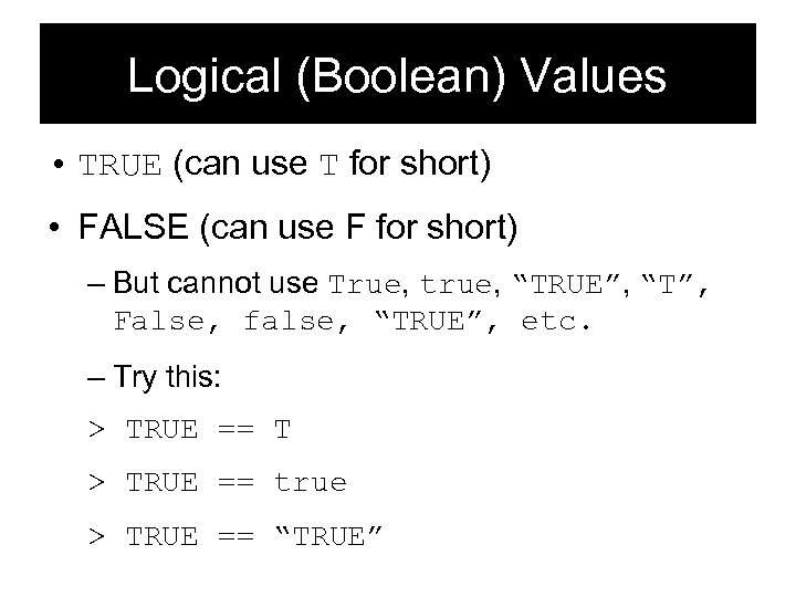Logical (Boolean) Values • TRUE (can use T for short) • FALSE (can use F for short) – But cannot use True, true, “TRUE”, “T”, False, false, “TRUE”, etc. – Try this: > TRUE == T > TRUE == true > TRUE == “TRUE”