ITT-Autumn-2016-Lecture-3-E.ppt
- Количество слайдов: 14
International Trade: Theory and Policy Lecture 3 September, 2016 Instructor: Natalia Davidson, Lecture is prepared by Prof. Sergey Kadochnikov, Natalia Davidson 1
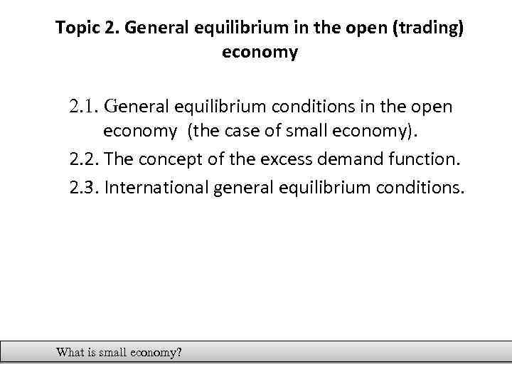
Topic 2. General equilibrium in the open (trading) economy 2. 1. General equilibrium conditions in the open economy (the case of small economy). 2. 2. The concept of the excess demand function. 2. 3. International general equilibrium conditions. What is small economy?
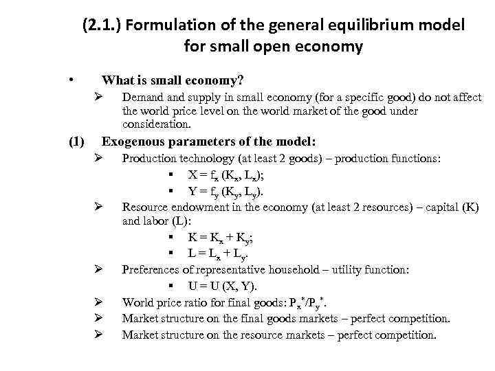
(2. 1. ) Formulation of the general equilibrium model for small open economy • What is small economy? Ø (1) Demand supply in small economy (for a specific good) do not affect the world price level on the world market of the good under consideration. Exogenous parameters of the model: Ø Ø Ø Production technology (at least 2 goods) – production functions: § Х = fx (Kx, Lx); § Y = fy (Ky, Ly). Resource endowment in the economy (at least 2 resources) – capital (K) and labor (L): § K = Kx + Ky; § L = Lx + Ly. Preferences of representative household – utility function: § U = U (X, Y). World price ratio for final goods: Px*/Py*. Market structure on the final goods markets – perfect competition. Market structure on the resource markets – perfect competition.
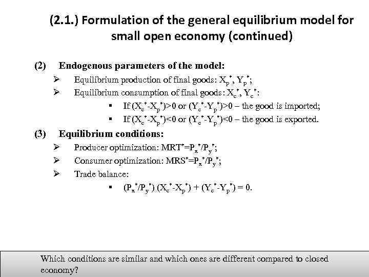
(2. 1. ) Formulation of the general equilibrium model for small open economy (continued) (2) Endogenous parameters of the model: Ø Ø (3) Equilibrium production of final goods: Xp*, Yp*; Equilibrium consumption of final goods: Xc*, Yc*: § If (Xc*-Xp*)>0 or (Yc*-Yp*)>0 – the good is imported; § If (Xc*-Xp*)<0 or (Yc*-Yp*)<0 – the good is exported. Equilibrium conditions: Ø Ø Ø Producer optimization: MRT*=Px*/Py*; Consumer optimization: MRS*=Px*/Py*; Trade balance: § (Px*/Py*) (Xc*-Xp*) + (Yc*-Yp*) = 0. Which conditions are similar and which ones are different compared to closed economy?
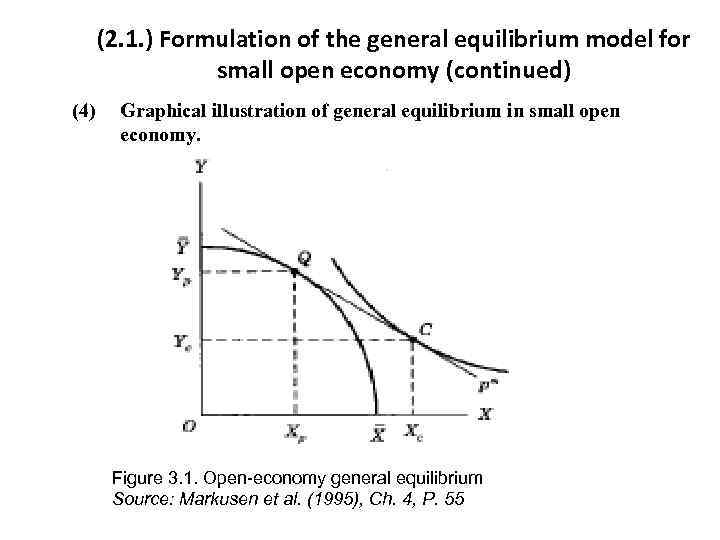
(2. 1. ) Formulation of the general equilibrium model for small open economy (continued) (4) Graphical illustration of general equilibrium in small open economy. Figure 3. 1. Open-economy general equilibrium Source: Markusen et al. (1995), Ch. 4, P. 55
(2. 2. ) The concept of the excess demand function • Definition (general): Ø The excess demand function: relates the world price ratio on the one hand difference between demand supply, on the other hand § Ex(Px/Py) = Xc(Px/Py) - Xp(Px/Py) • Graphical derivation of the excess demand function for small open economy: Ø From production possibilities curve of the economy
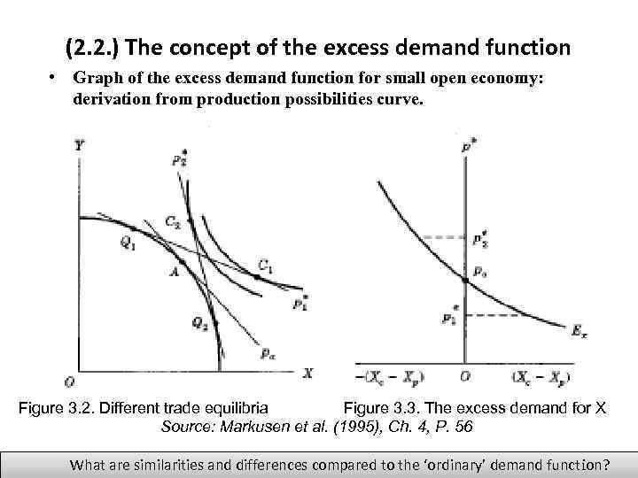
(2. 2. ) The concept of the excess demand function • Graph of the excess demand function for small open economy: derivation from production possibilities curve. Figure 3. 2. Different trade equilibria Figure 3. 3. The excess demand for X Source: Markusen et al. (1995), Ch. 4, P. 56 What are similarities and differences compared to the ‘ordinary’ demand function?
(2. 2. ) The concept of the excess demand function • Graph of the excess demand function for small open economy: characteristics Ø Slope of the excess demand curve; Ø Intersection with vertical axis.
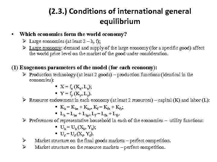
(2. 3. ) Conditions of international general equilibrium • Which economies form the world economy? Ø Large economies (at least 2 – h, f); Ø Large economy: demand supply of the large economy (for a specific good) affect the world price level on the market of the good under consideration. (1) Exogenous parameters of the model (for each economy): Ø Production technology (at least 2 goods) – production functions (identical in the economies): § Х = fx (Kx, Lx); § Y = fy (Ky, Ly). Ø Resource endowment in each economy (at least 2 resources) – capital (K) and labor (L): § Kh = Khx + Khy, Kf = Kfx + Kfy; § Lh = Lhx + Lhy, Lf = Lfx + Lfy. Ø Preferences of representative household in each of the economies – utility functions: § Uh = Uh (Xh, Yh); § Uf = Uf (Xf, Yf). Ø Market structure on the final goods markets – perfect competition. Ø Market structure on the resource markets – perfect competition.
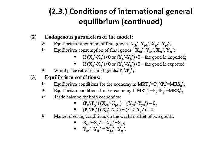
(2. 3. ) Conditions of international general equilibrium (continued) (2) Endogenous parameters of the model: Ø Ø Ø (3) Equilibrium production of final goods: Xph*, Yph*, Xpf*, Ypf*; Equilibrium consumption of final goods: Xсh*, Yсh*, Xсf*, Yсf*: § If (Xc*-Xp*)>0 or (Yc*-Yp*)>0 – the good is imported; § If (Xc*-Xp*)<0 or (Yc*-Yp*)<0 – the good is exported. World price ratio for final goods: Px*/Py*; Equilibrium conditions: Ø Ø Equilibrium conditions for the economy h: MRTh*=Px*/Py*=MRSh*; Equilibrium conditions for the economy f: MRTf*=Px*/Py*=MRSf*; Trade balance for both economies: § (Px*/Py*) (Xch*-Xph*) + (Ych*-Yph*) = 0; § (Px*/Py*) (Xcf*-Xpf*) + (Ycf*-Ypf*) = 0. Market clearing conditions on the world market of two goods: § Xch*+Xсf* = Xph*+Xpf; § Ych*+Yсf* = Yph*+Ypf*.
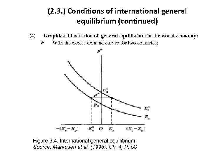
(2. 3. ) Conditions of international general equilibrium (continued) (4) Graphical illustration of general equilibrium in the world economy: Ø With the excess demand curves for two countries; Figure 3. 4. International general equilibrium Source: Markusen et al. (1995), Ch. 4, P. 58
(2. 3. ) Conditions of international general equilibrium (continued) (4) Graphical illustration of general equilibrium in the world economy: Ø With production possibility curves for two countries. During the lecture.

Homework (1) Exercise session 2 (2) Think about topics for reports during exercise sessions and work on a paper review (due 1 November 2016) Office hours: Friday 13: 50 – 14: 30, room 216. E-mail: natalya. davidson@gmail. com (Наталья Борисовна Давидсон) 13
Topic 3. The gains from free international trade under perfect competition on the markets 3. 1. Total gains from free international trade and the gains-from-trade theorem. 3. 2. The gains from specialization and the gains from exchange.
ITT-Autumn-2016-Lecture-3-E.ppt