International Trade : Theory and Policy Lecture 2

International Trade : Theory and Policy Lecture 2 September, 2016 Instructor: Natalia Davidson Lecture is prepared by Prof. Sergey Kadochnikov, Natalia Davidson, Irina Aleynikova

Topic 1. Issues of modern International Trade Theory. Technical concepts of International Trade Theory and general equilibrium in closed economy. 1. 1. Structure, problems and specific features of International Trade Theory. What is traded? Who is trading – countries or firms? In which sort of competition on global markets? 1. 2. General equilibrium of production sector in closed economy. Concept of technical and market efficiency in production. 1. 3. Interrelation between technology and production possibility curve. 1. 4. General equilibrium of household sector in closed economy. Concept of social indifference curves. 1. 5. General equilibrium in closed economy.

( 1. 4. ) General equilibrium of household sector in closed economy ( model of pure exchange economy ) (1) Exogenous parameters : Preferences of households ( at least 2 households ) – utility functions : U 1 = U 1 (X 1 , Y 1 ); U 2 = U 2 (X 2 , Y 2 ). Final goods endowments of households : X 0 = X 10 + X 20 ; Y 0 = Y 10 + Y 20. Market structure on the final goods markets – perfect competition. (2) Endogenous parameters : Equilibrium consumption of final goods by households : X 1* , X 2* , Y 1* , Y 2* ; Equilibrium relative prices of final goods – P x* / Py*. (3) Graphical illustration of exogenous parameters. (4) Graphical illustration of endogenous parameters of the model.

( 1. 4. ) Characteristics of the utility function General characteristics of the utility function : Substitution / complementarity between goods ; Homogeneity of the utility function ; Relative intensity of consumed goods. Specific features of the utility function in the model : Incomplete substitution / complementarity between goods in consumption; Homogeneous utility function of degree =< 1; Consumers differ in relative intensity of consumed goods. Graphical illustration of exogenous parameters. Pareto-optimality in household sector : Named for the Italian economist Vilfredo Pareto Final goods allocation among individuals is Pareto-optimal if in the event of any reallocation the utility of one individual’s choice cannot be increased without reducing the utility of at least one individual’s choice. See Graphical illustration of endogenous parameters.

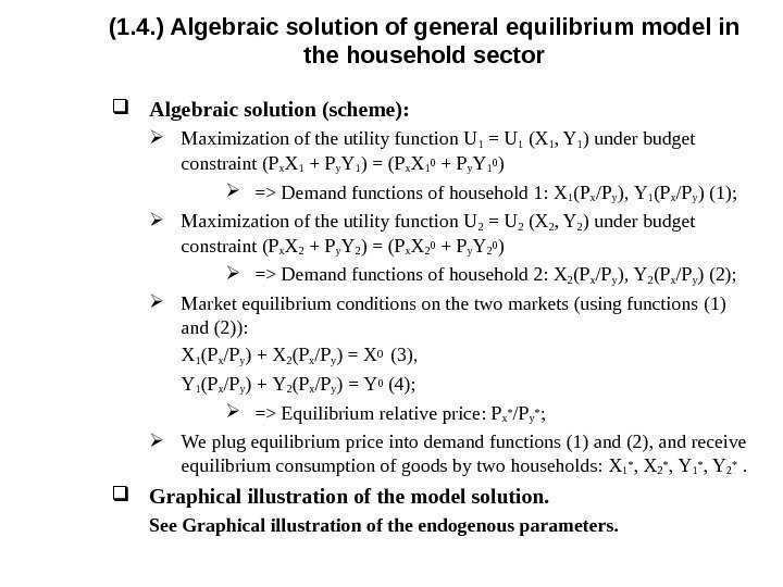
( 1. 4. ) Algebraic solution of general equilibrium model in the household sector Algebraic solution ( scheme ): Maximization of the utility function U 1 = U 1 (X 1 , Y 1 ) under budget constraint ( P x X 1 + P y Y 1 ) = ( P x X 1 0 + P y Y 1 0 ) => Demand functions of household 1: X 1 ( P x / P y ), Y 1 ( P x / P y ) (1); Maximization of the utility function U 2 = U 2 (X 2 , Y 2 ) under budget constraint ( P x X 2 + P y Y 2 ) = ( P x X 2 0 + P y Y 2 0 ) => Demand functions of household 2: X 2 ( P x / P y ), Y 2 ( P x / P y ) (2); Market equilibrium conditions on the two markets (using functions (1) and (2) ) : X 1 ( P x / P y ) + X 2 ( P x / P y ) = X 0 (3), Y 1 ( P x / P y ) + Y 2 ( P x / P y ) = Y 0 (4); => Equilibrium relative price : P x * / P y * ; We plug equilibrium price into demand functions (1) and (2), and receive equilibrium consumption of goods by two households : X 1 * , X 2 * , Y 1 * , Y 2 * . Graphical illustration of the model solution. See Graphical illustration of the endogenous parameters.

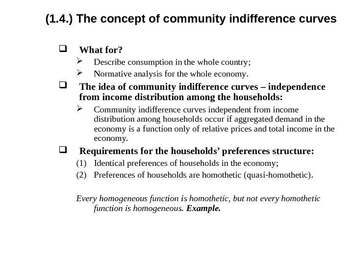
( 1. 4. ) The concept of community indifference curves What for ? Describe consumption in the whole country ; Normative analysis for the whole economy. The idea of community indifference curves – independence from income distribution among the households : Community indifference curves independent from income distribution among households occur if aggregated demand in the economy is a function only of relative prices and total income in the economy. Requirements for the households’ preferences structure : (1) Identical preferences of households in the economy ; (2) Preferences of households are homothetic (quasi-homothetic). Every homogeneous function is homothetic, but not every homothetic function is homogeneous. Example.

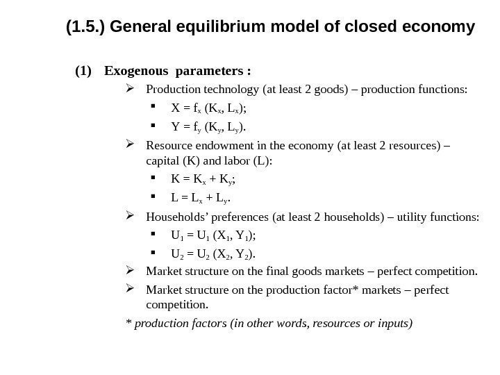
( 1. 5. ) General equilibrium model of closed economy (1) Exogenous parameters : Production technology ( at least 2 goods ) – production functions : Х = fx (Kx , Lx ); Y = f y (Ky , Ly ). Resource endowment in the economy ( at least 2 resources ) – capital ( K ) and labor ( L ): K = K x + Ky ; L = L x + Ly. Households’ preferences ( at least 2 households ) – utility functions : U 1 = U 1 (X 1 , Y 1 ); U 2 = U 2 (X 2 , Y 2 ). Market structure on the final goods markets – perfect competition. Market structure on the production factor* markets – perfect competition. * production factors (in other words, resources or inputs)

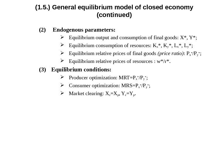
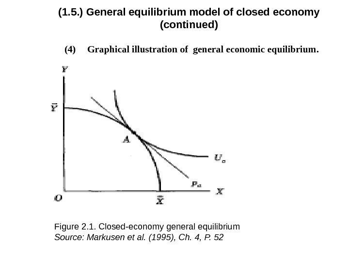
( 1. 5. ) General equilibrium model of closed economy (continued ) (2) Endogenous parameters : Equilibrium output and consumption of final goods : X*, Y*; Equilibrium consumption of resources : Kx *, Ky *, Lx *, Ly *; Equilibrium relative prices of final goods (price ratio) : P x* / Py* ; Equilibrium relative prices of resources : w*/r*. (3) Equilibrium conditions : Producer optimization : MRT=P x* / Py* ; Consumer optimization : MRS=P x* / Py* ; Market clearing : X c =Xp , Yc =Yp.

( 1. 5. ) General equilibrium model of closed economy (continued ) (4) Graphical illustration of general economic equilibrium. Figure 2. 1. Closed-economy general equilibrium Source : Markusen et al. (1995), Ch. 4, P.

Homework: (1) Exercise session 2 « General equilibrium of household sector and general equilibrium in closed economy » (2) Think about topics for reports during exercise sessions and start working on a paper review ( due 1 November 2016 ) Office hours: Friday 13: 50 – 14: 30, room 216. E-mail: natalya. davidson@gmail. com (Наталья Борисовна Давидсон)

Topic 2. General equilibrium in the open (trading) economy 2. 1. General equilibrium conditions in the open economy (the case of small economy). 2. 2. The concept of the excess demand function. 2. 3. International general equilibrium conditions.