Intelligently Principia Deciphering Unintelligible Biologica Design Bud

Intelligently Principia Deciphering Unintelligible Biologica Design

Bud Mishra Professor of Computer Science, Mathematics and Cell Biology ¦ Courant Institute, NYU School of Medicine, Tata Institute of Fundamental Research, and Mt. Sinai School of Medicine

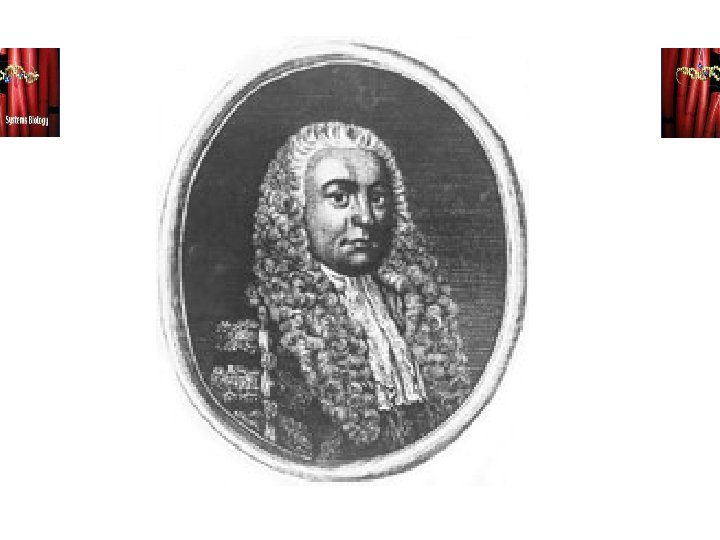
Robert Hooke • Robert Hooke (1635 -1703) was an experimental scientist, mathematician, architect, and astronomer. Secretary of the Royal Society from 1677 to 1682, … • Hooke was considered the “England’s Da Vinci” because of his wide range of interests. • His work Micrographia of 1665 contained his microscopical investigations, which included the first identification of biological cells. • In his drafts of Book II, Newton had referred to him as the most illustrious Hooke—”Cl[arissimus] Hookius. ” • Hooke became involved in a dispute with Isaac Newton over the priority of the discovery of the inverse square law of gravitation.

Hooke to Halley • “[Huygen’s Preface] is concerning those properties of gravity which I myself first discovered and showed to this Society and years since, which of late Mr. Newton has done me the favour to print and publish as his own inventions. “

Newton to Halley • “Now is this not very fine? Mathematicians that find out, settle & do all the business must content themselves with being nothing but dry calculators & drudges & another that does nothing but pretend & grasp at all things must carry away all the inventions… • “I beleive you would think him a man of a strange unsociable temper. ”

Newton to Hooke • “If I have seen further than other men, it is because I have stood on the shoulders of giants and you my dear Hooke, have not. " – Newton to Hooke

Image & Logic • The great distance between – a glimpsed truth and – a demonstrated truth • Christopher Wren/Alexis Claude Clairaut

Micrographia Principia

Micrographia

“The Brain & the Fancy” • “The truth is, the science of Nature has already been too long made only a work of the brain and the fancy. It is now high time that it should return to the plainness and soundness of observations on material and obvious things. ” – Robert Hooke. (1635 - 1703), Micrographia 1665

Principia

“Induction & Hypothesis” • “Truth being uniform and always the same, it is admirable to observe how easily we are enabled to make out very abstruse and difficult matters, when once true and genuine Principles are obtained. ” – Halley, “The true Theory of the Tides, extracted from that admired Treatise of Mr. Issac Newton, Intituled, Philosophiae Naturalis Principia Mathematica, ” Phil. Trans. 226: 445, 447. Hypotheses non fingo. I feign no hypotheses. Principia Mathematica. • This rule we must follow, that the argument of induction may not be evaded by hypotheses.

Morphogenesis

Alan Turing: 1952 • “The Chemical Basis of Morphogenesis, ” 1952, Phil. Trans. Roy. Soc. of London, Series B: Biological Sciences, 237: 37— 72. • A reaction-diffusion model for development.

“A mathematical model for the growing embryo. ” • A very general program for modeling embryogenesis: The `model’ is “a simplification and an idealization and consequently a falsification. ” • Morphogen: “is simply the kind of substance concerned in this theory…” in fact, anything that diffuses into the tissue and “somehow persuades it to develop along different lines from those which would have been followed in its absence” qualifies.

Diffusion equation first temporal derivative: rate ¶ a/¶ t = Da r 2 a a: concentration Da: diffusion constant second spatial derivative: flux

Reaction-Diffusion ¶a/¶ t = f(a, b) + Da r 2 a f(a, b) = a(b-1) –k 1 ¶ b/¶ t = g(a, b) + Db r 2 b g(a, b) = -ab +k 2 Turing, A. M. (1952). “The chemical basis of morphogenesis. “ Phil. Trans. Roy. Soc. London B 237: 37 a - b reaction diffusion

Reaction-diffusion: an example A fed at rate F d[A]/dt=F(1 -[A]) A+2 B ! 3 B B!P B extracted at rate F, decay at rate k d[B]/dt=-(F+k)[B] reaction: -d[A]/dt = d[B]/dt = [A][B]2 diffusion: d[A]/dt=DA 2[A]; d[B]/dt=DB 2[B] ¶ [A]/¶ t = F(1 -[A]) – [A][B]2 + DA 2[A] ¶ [B]/¶ t = -(F+k)[B] +[A][B]2 + DB 2[B] Pearson, J. E. : Complex patterns in simple systems. Science 261, 189 -192 (1993).

Reaction-diffusion: an example

Genes: 1952 • Since the role of genes is presumably catalytic, influencing only the rate of reactions, unless one is interested in comparison of organisms, they “may be eliminated from the discussion…”

Crick & Watson : 1953

Genome • Genome: – Hereditary information of an organism is encoded in its DNA and enclosed in a cell (unless it is a virus). All the information contained in the DNA of a single organism is its genome. • DNA molecule can be thought of as a very long sequence of nucleotides or bases: S = {A, T, C, G}

The Central Dogma • DNA Transcription RNA Translation The central dogma(due to Francis Crick in 1958) states that these information flows are all unidirectional: “The central dogma states that once `information' has passed into protein it cannot get out again. The transfer of information from nucleic acid to nucleic acid, or from nucleic acid to protein, may be possible, but transfer from protein to protein, or from protein to nucleic acid is impossible. Information means here the precise determination of sequence, either of bases in the Protein nucleic acid or of amino acid residues in the protein. ”

RNA, Genes and Promoters • • • Promoter A specific region of DNA that determines the synthesis of proteins (through the transcription and translation) is called a gene – Originally, a gene meant something more abstract---a unit of hereditary inheritance. – Now a gene has been given a physical molecular existence. Transcription of a gene to a messenger RNA, m. RNA, is keyed by a transcriptional activator/factor, which attaches to a promoter (a specific sequence adjacent to the gene). Regulatory sequences such as silencers and enhancers control the rate of transcription Terminator 10 -35 bp Transcriptional Initiation Gene Transcriptional Termination

“The Brain & the Fancy” “Work on the mathematics of growth as opposed to the statistical description and comparison of growth, seems to me to have developed along two equally unprofitable lines… It is futile to conjure up in the imagination a system of differential equations for the purpose of accounting for facts which are not only very complex, but largely unknown, …What we require at the present time is more measurement and less theory. ” – Eric Ponder, Director, CSHL (LIBA), 19361941.

“Axioms of Platitudes” -E. B. Wilson 1. Science need not be mathematical. 2. Simply because a subject is mathematical it need not therefore be scientific. 3. Empirical curve fitting may be without other than classificatory significance. 4. Growth of an individual should not be confused with the growth of an aggregate (or average) of individuals. 5. Different aspects of the individual, or of the average, may have different types of growth curves.

Genes for Segmentation • Fertilization followed by cell division • Pattern formation – instructions for – Body plan (Axes: A-P, D-V) – Germ layers (ecto-, meso-, endoderm) • Cell movement - form – gastrulation • Cell differentiation

PI: Positional Information • Positional value – Morphogen – a substance – Threshold concentration • Program for development – Generative rather than descriptive • “French-Flag Model”

bicoid • The bicoid gene provides an A-P morphogen gradient

gap genes • The A-P axis is divided into broad regions by gap gene expression • The first zygotic genes • Respond to maternallyderived instructions • Short-lived proteins, gives bell-shaped distribution from source

Transcription Factors in Cascade • Hunchback (hb) , a gap gene, responds to the dose of bicoid protein • A concentration above threshold of bicoid activates the expression of hb • The more bicoid transcripts, the further back hb expression goes

Transcription Factors in Cascade • Krüppel (Kr), a gap gene, responds to the dose of hb protein • A concentration above minimum threshold of hb activates the expression of Kr • A concentration above maximum threshold of hb inactivates the expression of Kr

Segmentation • Parasegments are delimited by expression of pairrule genes in a periodic pattern • Each is expressed in a series of 7 transverse stripes

Pattern Formation – Edward Lewis, of the California Institute of Technology – Christiane Nuesslein-Volhard, of Germany's Max-Planck Institute – Eric Wieschaus, at Princeton • Each of the three were involved in the early research to find the genes controlling development of the Drosophila fruit fly.

The Network of Interaction EN CID CN hh proteins WG positive interacions en PTC PH PH HH a cell m. RNA WG PTC ptc + cid wg en HH Cell-to-cell interface negative interacions a neighbor Legend: • WG=wingless • HH=hedgehog • CID=cubitus iterruptus • CN=repressor fragment of CID • PTC=patched • PH=patchedhedgehog complex

Completeness • “We incorporated these two remedies first (light gray lines). With these links installed there are many parameter sets that enable the model to reproduce the target behavior, so many that they can be found easily by random sampling. ”

Model Parameters

Complete Model

Is this your final answer? • • It is not uncommon to assume certain biological problems to have achieved a cognitive finality without rigorous justification. Rigorous mathematical models with automated tools for reasoning, simulation, and computation can be of enormous help to uncover – cognitive flaws, – qualitative simplification or – overly generalized assumptions. • Some ideal candidates for such study would include: – – prion hypothesis cell cycle machinery muscle contractility processes involved in cancer (cell cycle regulation, angiogenesis, DNA repair, apoptosis, cellular senescence, tissue space modeling enzymes, etc. ) – signal transduction pathways, and many others.

Computational Systems Biology

Systems Biology Combining the mathematical rigor of numerology with the predictive power of astrology. Cyberia Numerlogy SYSTEMS BIOLOGY The Astrology Numeristan HOTzone Astrostan Infostan Interpretive Biology Integrative Biology Computational Biology Bioinformatics Bio. Spice

Why do we need a tool? We claim that, by drawing upon mathematical approaches developed in the context of dynamical systems, kinetic analysis, computational theory and logic, it is possible to create powerful simulation, analysis and reasoning tools for working biologists to be used in deciphering existing data, devising new experiments and ultimately, understanding functional properties of genomes, proteomes, cells, organs and organisms. Simulate Biologists! Not Biology!!

Future Biology of the future should only involve a biologist and his dog: the biologist to watch the biological experiments and understand the hypotheses that the data-analysis algorithms produce and the dog to bite him if he ever touches the experiments or the computers.

Simpathica is a modular system Canonical Form: Characteristics: • Predefined Modular Structure • Automated Translation from Graphical to Mathematical Model • Scalability

Glycolysis Glycogen P_i Glucose-1 -P Phosphorylase a Phosphoglucomutase Glucokinase Glucose-6 -P Phosphoglucose isomerase Fructose-6 -P Phosphofructokinase

Formal Definition of S-system

An Artificial Clock • Three proteins: – Lac. I, tet. R & l c. I – Arranged in a cyclic manner (logically, not necessarily physically) so that the protein product of one gene is rpressor for the next gene. Lac. I! : tet. R; tet. R! Tet. R! : l c. I; l c. I ! l c. I! : lac. I; lac. I! Lac. I Leibler et al. , Guet et al. , Antoniotti et al. , Wigler & Mishra

Biological Model • Standard molecular biology: Construct – A low-copy plasmid encoding the repressilator and – A compatible higher-copy reporter plasmid containing the tetrepressible promoter PLtet 01 fused to an intermediate stability variant of gfp.

Cascade Model: Repressilator? x 1 - dx 2/dt = a 2 X 6 g 26 X 1 g 21 - b 2 X 2 h 22 dx 4/dt = a 4 X 2 g 42 X 3 g 43 - b 4 X 4 h 44 dx 6/dt = a 6 X 4 g 64 X 5 g 65 - b 6 X 6 h 66 X 1, X 3, X 5 = const x 2 x 3 - x 4 x 5 - x 6

Sim. Pathica System

Simpathica System Model Simulation Model Building Model Checking

Algebraic Approaches

Differential Algebra

Example System

Input-Output Relations

Obstacles

Simpler Computational Models • Kripke Models/Discrete Event Systems • Hybrid Automata • Their Connection to – Turing Machines – “Real” Turing Machines

Kripke Structure • Formal Encoding of a Dynamical System: • Simple and intuitive pictorial representation of the behavior of a complex system – A Graph with nodes representing system states labeled with information true at that state – The edges represent system transitions as the result of some action

Computation Tree G 0 [b] G 1 M S G G 0 G 1 G 2 [a] G G 0 G 1 M 0 S M S 0 G 2 S M G 2 M G 1 G G 0 G 1 M 0 S M • Finite set of states; Some are initial states • Total transition relation: every state has at least one next state i. e. infinite paths • There is a set of basic environmental variables or features (“atomic propositions”) • In each state, some atomic propositions are true

Hybrid Automata

Thermostat

Intuition

Semantics

Engineered Systems

Chemotaxis • Escherichia coli has evolved a strategy for responding to a chemical gradient in its environment – It detects the concentration of ligands through a number of receptors – It reacts by driving its flagella motors to alter its path of motion. – Either it “runs” – moves in a straight line by moving its flagella counterclockwise (CCW), or it “tumbles” – randomly change its heading by moving its flagella clockwise (CW). • • The response is mediated through the molecular concentration of Che. Y in a phosphorylated form, which in turn is determined by the bound ligands at the receptors that appear in several forms. The more detailed pathway involves other – – • Che. B (either with phosphorylation or without, Bp and B 0), Che. Z (Z), bound receptors (LT) and unbound receptors (T) Their continuous evolution is determined by a set of differential algebraic equations derived through kinetic mass action formulation.

Non-Stochastic Chemotaxis

Questions of Interest • Controllability: – Assume that the system is at the “origin” initially. Can we find a control signal so that the state reaches a given position at a fixed time? • Observability: – Can the state x be determined from observations of the output y over some time interval. • Reachability: A computationally simpler problem: – Can we determine what states are reached as the system evolves autonomously or under a class of control signal. • “HALTING” Problem: – Can the system reach a designated state at some time and then stay there?

Decision problems

Dynamics • Replacing differential equations by “equivalent” dynamics:

Two New Models

First Order Theory of Reals • Tarski's theorem says that the first-order theory of reals with +, £, =, and > allows quantifier elimination. Algorithmic quantifier elimination implies decidability. • Every quantifier-free formula composed of polynomial equations and inequalities, and Boolean connectives defines a semialgebraic set. Thus a set S is semi-algebraic if:

Sa. Co. Re • Hybrid Automata’s inclusion dynamics, approximated by semi-algebraic formula. Dyn[X, X’, T] ´ Semialgebraic Set • A more realistic approximation, for time invariant systems: – Dyn[X, X’, h] ¼ {X’ | X’ = X + F(X, 0) h + d, |d| < e}, for a suitably chosen e ´ |F’(X, 0) h 2/2! + F’(X, 0) h 3/3! + L |

Another Example: Biological Pattern Formation • Embryonic Skin Of The South African Claw. Toed Frog • “Salt-and-Pepper” pattern formed due to lateral inhibition in the Xenopus epidermal layer

Delta-Notch Signalling Physically adjacent cells laterally inhibit each other’s ciliation (Delta production)

Delta-Notch Pathway • Delta binds and activates its receptor Notch in neighboring cells (proteolytic release and nuclear translocation of the intracellular domain of Notch) • Activated Notch suppresses ligand (Delta) production in the cell • A cell producing more ligands forces its neighboring cells to produce less

Pattern formation by lateral inhibition with feedback: a mathematical model of Delta-Notch intercellular signalling Collier et al. (1996) Rewriting… Where: Collier et al.

One-Cell Delta-Notch Hybrid Automaton Q 1 Q 2 Both OFF Delta ON Q 3 Q 4 Notch ON Both ON Ghosh et al.

Two-Cell Delta-Notch System Q 1 Q 2 Neither Delta Q 3 Q 4 Notch Both Cell 1 Q 1 Q 2 Neither Delta 16 Discrete States Cell 2

System Properties: True & Approximate Q 3 Q 2 Notch Delta Q 2 Q 3 Delta Notch

State Reachability Q 2 Q 3 Delta Notch

State Reachability Q 3 Q 2 Notch Delta

Impossibility Of Reaching Wrong Equilibrium: Q 2 Delta Q 3 Notch

Hybrid Hierarchy

Logic & Model-Checking

Deciphering Design Principles in a Biological Systems Step 1. Formally encode the behavior of the system as a hybrid automaton Step 2. Formally encode the properties of interest in a powerful logic Step 3. Automate the process of checking if the formal model of the system satisfies the formally encoded properties using Model Checking

Temporal Logic • First Order Logic: Time is an explicitly quantified variable • Propositional Modal logic: was invented to formalize modal notions and suppress the quantified variables – with operators “possibly P” and “necessarily P” (similar to “eventually” and “henceforth”)

Branching versus Linear Time • • • Temporal Logic: – Short hand for describing the way properties of the system change with time – Time is implicit Linear-time: Only one possible future in a moment – Look at individual computations Branching-time: It may be possible to split to different courses depending on possible futures – Look at the tree of computations Time is Linear Time is Branching

Computation Tree Logic (CTL) • Branching Time temporal logic: interpreted over an execution tree where branching denotes non-deterministic actions • Explicitly quantify over two modes – the path and the time • Each time we talk about a temporal property, we also specify whether it is true on all possible paths or whether it is true on at least one path - Path quantifiers – A = “for all future paths” – E = “for some future path”

Semantics for CTL • For p AP: s ² p p L(s) • s ² f Æ g s ² f and s ² g • s ² f Ç g s ² f or s ² g • s ² EX f =hs 0 s 1. . . i from s s 1 ² f • s ² E(f U g) = hs 0 s 1. . . i from s j 0 [ sj ² g and i : 0 i j [si ² f ] ] • s ² EG f = hs 0 s 1. . . i from s i 0: si ² f

Some CTL Operators EF g AF g EG g AG g

CTL Model-Checking • Straight-forward approach: Recursive descent on the structure of the query formula • Label the states with the terms in the formula: – Proceed by marking each point with the set of valid subformulas • “Global” algorithm: – Iterate on the structure of the property, traversing the whole of the model in each step – Use fixed point unfolding to interpret Until:

Naïve CTL Model-Checker

Other Model Checking Algorithms • LTL Model Checking: Tableu-based… • CTL* Model Checking: Combine CTL and LTL Model Checkers… • Symbolic Model Checking – – Binary Decision Diagram OBDD-based model-checking for CTL Fixed-point Representation Automata-based LTL Model-Checking • SAT-based Model Checking • Algorithmic Algebraic Model Checking • Hierarchical Model Checking

Purine Metabolism • Purine Metabolism – Provides the organism with building blocks for the synthesis of DNA and RNA. – The consequences of a malfunctioning purine metabolism pathway are severe and can lead to death. • The entire pathway is almost closed but also quite complex. It contains – several feedback loops, – cross-activations and – reversible reactions • Thus is an ideal candidate for reasoning with computational tools.

Simple Model

Biochemistry of Purine Metabolism • The main metabolite in purine biosynthesis is 5 -phosphoribosyl-a-1 pyrophosphate (PRPP). – A linear cascade of reactions converts PRPP into inosine monophosphate (IMP). IMP is the central branch point of the purine metabolism pathway. – IMP is transformed into AMP and GMP. – Guanosine, adenosine and their derivatives are recycled (unless used elsewhere) into hypoxanthine (HX) and xanthine (XA). – XA is finally oxidized into uric acid (UA).

Purine Metabolism

Queries • Variation of the initial concentration of PRPP does not change the steady state. (PRPP = 10 * PRPP 1) implies steady_state() • This query will be true when evaluated against the modified simulation run (i. e. the one where the initial concentration of PRPP is 10 times the initial concentration in the first run – PRPP 1). TRUE • • Persistent increase in the initial concentration of PRPP does cause unwanted changes in the steady state values of some metabolites. If the increase in the level of PRPP is in the order of 70% then the system does reach a steady state, and we expect to see increases in the levels of IMP and of the hypoxanthine pool in a “comparable” order of magnitude. Always (PRPP = 1. 7*PRPP 1) implies steady_state() TRUE

Queries • Consider the following statement: • Eventually (Always (PRPP = 1. 7 * PRPP 1) implies steady_state() and Eventually Always(IMP < 2* IMP 1)) and Eventually (Always (hx_pool < 10*hx_pool 1))) • where IMP 1 and hx_pool 1 are the values observed in the unmodified trace. The above statement turns out to be false over the modified experiment trace. . • • False In fact, the increase in IMP is about 6. 5 fold while the hypoxanthine pool increase is about 60 fold. Since the above queries turn out to be false over the modified trace, we conclude that the model “over-predicts” the increases in some of its products and that it should therefore be amended

Final Model

Purine Metabolism

Continuous-Time Logics • Linear Time – – – Metric Temporal Logic (MTL) Timed Propositional Temporal Logic (TPTL) Real-Time Temporal Logic (RTTL) Explicit-Clock Temporal Logic (ECTL) Metric Interval Temporal Logic (MITL) • Branching time – Real-Time Computation Tree Logic (RTCTL) – Timed Computation Tree Logic (TCTL) Alur et al,

TCTL: Syntax And Semantics

T-μ CALCULUS: Syntax

“Until”: T- μ Fixpoint • s 2 is true now or • s 1 holds for one-step on some path after which s 2 holds or • s 1 holds for one-step on some path after which s 1 holds for one more step on some path after which s 2 holds or • and so on. .

TCTL Model Checking • Only “Until” requires “computation” • Until: Iterative computation of “onestep” Until • Least fixpoint computation:

Semi-Decidability Of TCTL • Global “time” variable – Allows interpretation of the TCTL operators freeze (z. X) and subscripted until (Ua) • While “one-step until” is decidable, the fixpoint is not guaranteed to converge • So TCTL is “semi”-decidable

Mandelbrot Hybrid Automaton Let: Invariant: False Then: Flows: Null Reachability Query:

Solution • Bounded Model Checking – Fully O-minimal Systems for Dense CTL • Constrained Systems – Linear Systems for Dense CTL – O-minimal for Dense CTL – SACo. Re (Semi algebraic Constrained Reset) for TCTL – IDA (Independent Dynamics Automata) for TCTL

Hooke Thursday 25 May 1676 Damned Doggs. Vindica me deus. • Commenting on Sir Nicholas Gimcrack character in The Virtuoso, a play by Thomas Shadwell.

Hooke in the Royal Society, 26 June 1689 • “And though many things I have first Discovered could not find acceptance yet I finde there are not wanting some who pride themselves on arrogating of them for their own… • “—But I let that passe for the present. ”

Hooke… • “So many are the links, upon which the true Philosophy depends, of which, if any can be loose, or weak, the whole chain is in danger of being dissolved; • “it is to begin with the Hands and Eyes, and to proceed on through the Memory, to be continued by the Reason; • “nor is it to stop there, but to come about to the Hands and Eyes again, and so, by a continuall passage round from one Faculty to another, it is to be maintained in life and strength. ”

The end…