68194ef311883ed092e6b03f604af74b.ppt
- Количество слайдов: 21
 Integrating Cost and Schedule Estimation In The COSYSMOR Model/Tool John E. Gaffney, Jr. 301 -721 -5710 j. gaffney@lmco. com Center For Process Improvement Excellence Corporate Engineering and Technology Lockheed Martin Corporation November 3, 2009 11/03/09 (c) Copyright Lockheed Martin Corporation 2009 1
 Focus Issues and Questions-1 • An issue of considerable importance to proposal managers, program managers, technical planners and to software engineering and systems engineering managers is how schedule compression or stretch-out* affects engineering costs or overall project costs • They are also interested in the opposite question, how engineering costs affect schedule. Indeed, a project might be cost driven or schedule driven or some combination of the two. More generally, managers and other stakeholders cited above are interested in the relationship between cost and schedule (project duration). • Thus, cost can imply schedule or vice versa. *Schedule compression (or stretch-out) can be defined as the amount or percentage of reduction (increase) of a project or software or systems engineering schedule with respect to some ideal or nominal value as related to cost or productivity 11/03/09 (c) Copyright Lockheed Martin Corporation 2009 2
 Focus Issues and Questions-2 • Knowing the relation between cost and schedule can help us to answer questions such as: 1. What is the schedule corresponding to this (estimated) cost value? 2. What is the (estimated) cost value corresponding to this schedule value? 3. Can cost and schedule be traded off (can one “buy off” the other)? Sometimes this is possible, and sometimes, it is not 11/03/09 (c) Copyright Lockheed Martin Corporation 2009 3
 Background/Reference To Earlier Work • • • The approach described here has been implemented in the COSYSMOR (“COSYSMO Risk and Reuse”) tool and the COCOMOR (“COCOMO Risk”) tool developed at Lockheed Martin. COSYSMOR evolved from the COSYSMO tool, developed by Dr. Ricardo Valerdi, and is available to anyone upon request. COSYSMOR was described at the 23 rd International COCOMO forum in October, 2008 More generally, the approach presented applies to estimating models such as COSYSMO and COCOMO that produce cost (labor) estimates as their principal outputs This presentation expands upon work described in a talk given at the 23 rd International COCOMO forum in October, 2008 by John Gaffney , and in a talk (and paper) given at the 7 th Annual Conference on Systems Engineering Research 2009 (CSER 2009), by John Gaffney, Ricardo Valerdi, and Michael Ross. Dr. Valerdi gave the presentation. The former was “Looking At Schedule Vs. Effort In Software Engineering, Systems Engineering and Systems. ” The latter was “Approaches to Calculating Systems Engineering Schedule in Parametric Cost Models” 11/03/09 (c) Copyright Lockheed Martin Corporation 2009 4
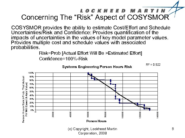 Concerning The “Risk” Aspect of COSYSMOR provides the ability to estimate Cost/Effort and Schedule Uncertainties/Risk and Confidence: Provides quantification of the impacts of uncertainties in the values of key model parameter values. Provides multiple cost and schedule values with associated probabilities. Risk=Prob [Actual Effort Will Be >Estimated Effort] Confidence=100%-Risk R 2 = 0. 9222 Systems Engineering Person Hours Risk 90% 80% 70% 60% 50% 40% 30% 20% 140000 120000 100000 80000 60000 40000 20000 0% 0 Person Hours Risk (=Prob. That Actual PH Will Exeed X-Axis Value) 100% Person Hours (c) Copyright, Lockheed Martin Corporation, 2008 5
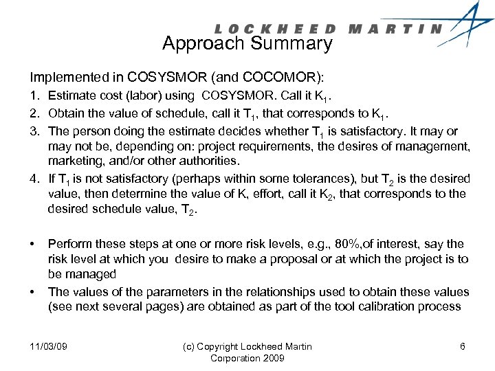 Approach Summary Implemented in COSYSMOR (and COCOMOR): 1. Estimate cost (labor) using COSYSMOR. Call it K 1. 2. Obtain the value of schedule, call it T 1, that corresponds to K 1. 3. The person doing the estimate decides whether T 1 is satisfactory. It may or may not be, depending on: project requirements, the desires of management, marketing, and/or other authorities. 4. If T 1 is not satisfactory (perhaps within some tolerances), but T 2 is the desired value, then determine the value of K, effort, call it K 2, that corresponds to the desired schedule value, T 2. • • Perform these steps at one or more risk levels, e. g. , 80%, of interest, say the risk level at which you desire to make a proposal or at which the project is to be managed The values of the parameters in the relationships used to obtain these values (see next several pages) are obtained as part of the tool calibration process 11/03/09 (c) Copyright Lockheed Martin Corporation 2009 6
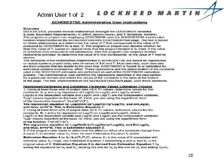
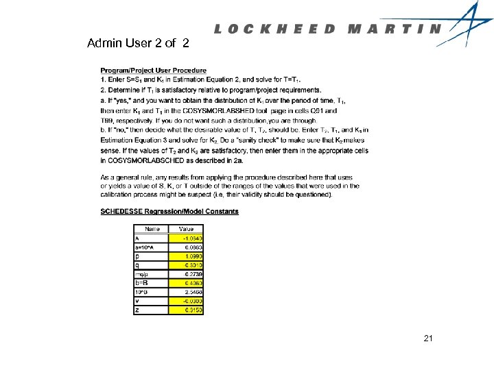
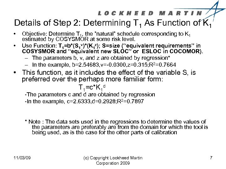 Details of Step 2: Determining T 1 As Function of K 1 • • Objective: Determine T 1, the ”natural” schedule corresponding to K 1 estimated by COSYSMOR at some risk level. Use Function: T 1=b*(S 1 v)*(K 1 z); S=size (“equivalent requirements” in COSYSMOR and “equivalent new SLOC” or ESLOC in COCOMOR). – The parameters b, v, and z are obtained by regression* – In the example, b=2. 54683, v=-0. 0300, z=0. 315; R 2=0. 7664 • This function, as it includes the effect of the variable S, is preferred over the perhaps more familiar form: T 1=c*K 1 d -The parameters c and d are obtained by regression -In the example, c=2. 6333, d=0. 2928; R 2=0. 7897 * Note : The data sets used in the regressions to determine the values of the parameters are preferably are from the domain for which the tool is being used, as is the case for the other parts of calibration 11/03/09 (c) Copyright Lockheed Martin Corporation 2009 7
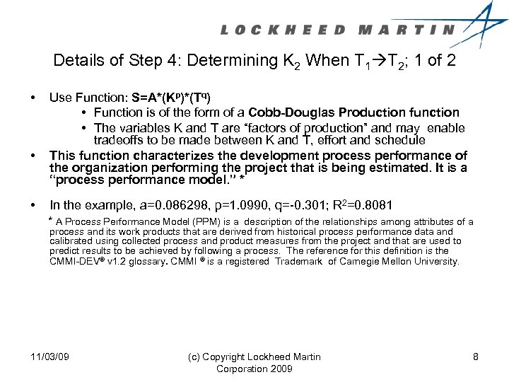 Details of Step 4: Determining K 2 When T 1 T 2; 1 of 2 • • • Use Function: S=A*(Kp)*(Tq) • Function is of the form of a Cobb-Douglas Production function • The variables K and T are “factors of production” and may enable tradeoffs to be made between K and T, effort and schedule This function characterizes the development process performance of the organization performing the project that is being estimated. It is a “process performance model. ” * In the example, a=0. 086298, p=1. 0990, q=-0. 301; R 2=0. 8081 * A Process Performance Model (PPM) is a description of the relationships among attributes of a process and its work products that are derived from historical process performance data and calibrated using collected process and product measures from the project and that are used to predict results to be achieved by following a process. The reference for this definition is the CMMI-DEV® v 1. 2 glossary. CMMI ® is a registered Trademark of Carnegie Mellon University. 11/03/09 (c) Copyright Lockheed Martin Corporation 2009 8
 Details of Step 4: Determining K 2 When T 1 T 2; 2 of 2 • • • Consider two instances:
 and ; Write: S 2/S 1 and then for S 1=S 2, we have: 1=((K 2/K 1)p)*((T 2/T 1)q). This can be rewritten as: ((K 2/K 1)p)=1/((T 2/T 1)q) and setting q/p=r, we obtain: (K 2/K 1)=1/((T 2/T 1)r ; Recalling p=1. 0990, q=-0. 301, the r=q/p=-0. 273885 Thus, to estimate the affect on K , effort, if the schedule were to be changed from T 1 to a more desirable value, T 2, use this relationship to obtain the “new” value of K, K 2; that is: K 2=K 1/((T 2/T 1)r; 11/03/09 (c) Copyright Lockheed Martin Corporation 2009 9
 COSYSMOR Effort/Schedule Inputs and Outputs 10
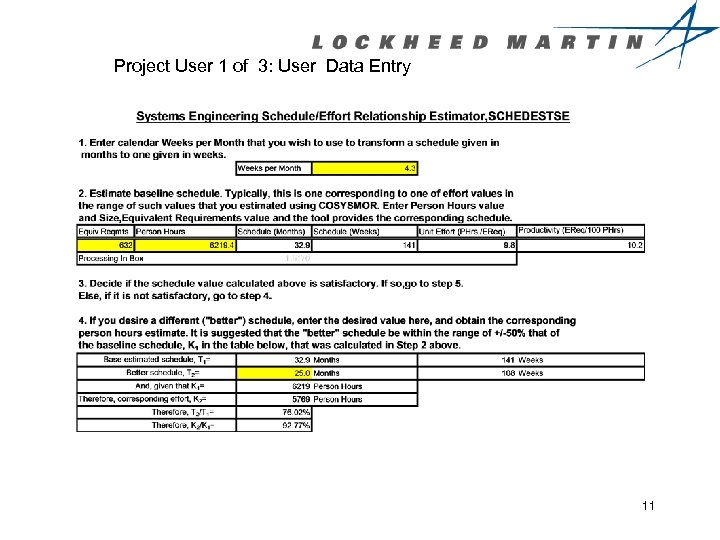 Project User 1 of 3: User Data Entry 11
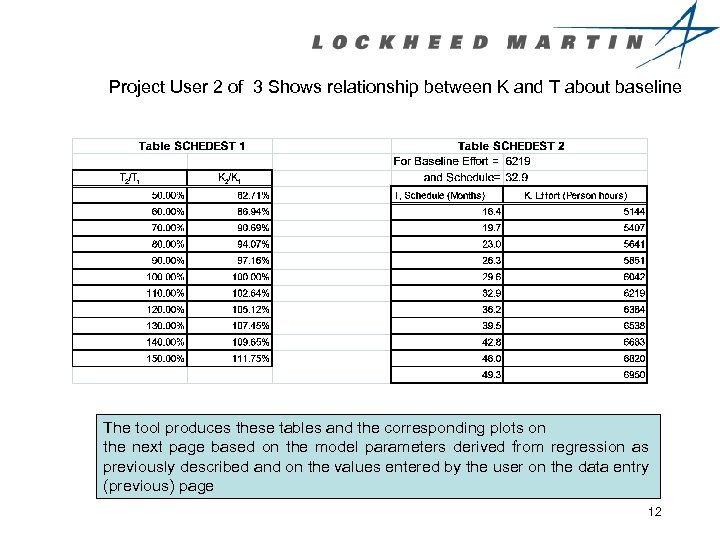 Project User 2 of 3 Shows relationship between K and T about baseline The tool produces these tables and the corresponding plots on the next page based on the model parameters derived from regression as previously described and on the values entered by the user on the data entry (previous) page 12
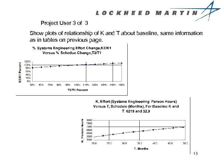 Project User 3 of 3 Show plots of relationship of K and T about baseline, same information as in tables on previous page. 13
 Summary • Determining the relationship between schedule and effort is important for project planning and management – A project may be effort (cost) or schedule driven or some combination of both • COSYSMOR can provide such a relationship – This enables sensitivities in effort/ and schedule to be evaluated • A production equation of the form: S=A*(Kp)*(Tq) is employed as part of the tool calibration process – The production function defines the ability of the organization for a certain domain to produce S as a function of the “factors of production, ” K and T. – The methodology can be used in other venues, such as software development and for businesses more generally, say to produce a certain sales volume as a function of labor applied and invested capital 3/18/201811/03/09 14
 Backup 15
 Cobb-Douglas Production Function • The Cobb-Douglas Production Function relates an output of a process to factors of production – An example is a C-D P F that relates software source statements, S, produced by a software development process, to factors of production, such as labor, K, and time or project duration, T – General Form: O=A*(F 1 Q 1)*(F 2 Q 2)*…. . *(FNQN); O=Output; the Fi are the factors of production • Examples of Use of the Production Function Form – Inputs: labor and capital; output=automobiles. From this form can be derived a “productivity, ” actually a “unit cost, ” labor hours per automobile. Notice the indicated possible tradeoff between capital (appropriately applied in terms of training and technology) and labor; more capital less labor to obtain the same output – Inputs: invested capital, labor; output=$ profit From this form can be derived a “productivity, ” return-on-invested capital” – Inputs: invested capital, labor; output=$ sales From this form can be derived a “productivity, ” “sales per employee” – Inputs: inspection time, meeting time, amount of material inspected; output= number of defects discovered. Can use as a basis for “tuning” the inspection process and for identifying opportunities for process improvement 11/03/09 (c) Copyright Lockheed Martin Corporation 2009 16
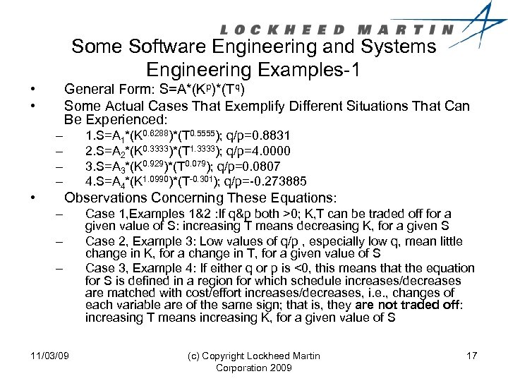 Some Software Engineering and Systems Engineering Examples-1 • • General Form: S=A*(Kp)*(Tq) Some Actual Cases That Exemplify Different Situations That Can Be Experienced: – – • 1. S=A 1*(K 0. 6288)*(T 0. 5555); q/p=0. 8831 2. S=A 2*(K 0. 3333)*(T 1. 3333); q/p=4. 0000 3. S=A 3*(K 0. 929)*(T 0. 079); q/p=0. 0807 4. S=A 4*(K 1. 0990)*(T-0. 301); q/p=-0. 273885 Observations Concerning These Equations: – – – 11/03/09 Case 1, Examples 1&2 : If q&p both >0; K, T can be traded off for a given value of S: increasing T means decreasing K, for a given S Case 2, Example 3: Low values of q/p , especially low q, mean little change in K, for a change in T, for a given value of S Case 3, Example 4: If either q or p is <0, this means that the equation for S is defined in a region for which schedule increases/decreases are matched with cost/effort increases/decreases, i. e. , changes of each variable are of the same sign; that is, they are not traded off: increasing T means increasing K, for a given value of S (c) Copyright Lockheed Martin Corporation 2009 17
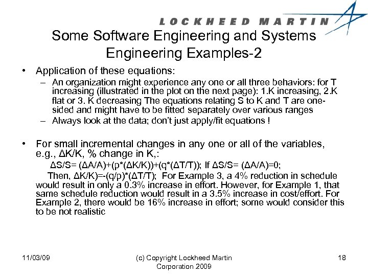 Some Software Engineering and Systems Engineering Examples-2 • Application of these equations: – An organization might experience any one or all three behaviors: for T increasing (illustrated in the plot on the next page): 1. K increasing, 2. K flat or 3. K decreasing The equations relating S to K and T are onesided and might have to be fitted separately over various ranges – Always look at the data; don’t just apply/fit equations ! • For small incremental changes in any one or all of the variables, e. g. , ΔK/K, % change in K, : ΔS/S= (ΔA/A)+(p*(ΔK/K))+(q*(ΔT/T)); If ΔS/S= (ΔA/A)=0; Then, ΔK/K)=-(q/p)*(ΔT/T); For Example 3, a 4% reduction in schedule would result in only a 0. 3% increase in effort. However, for Example 1, that same schedule reduction would result in a 3. 5% increase in cost/effort. For Example 2, there would be 16% increase in effort; some would consider this to be not realistic 11/03/09 (c) Copyright Lockheed Martin Corporation 2009 18
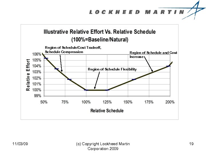 Region of Schedule/Cost Tradeoff, Schedule Compression Region of Schedule and Cost Increase Region of Schedule Flexibility 11/03/09 (c) Copyright Lockheed Martin Corporation 2009 19
 Admin User 1 of 2 20
 Admin User 2 of 2 21


