306796cb38611f7be5968e6b3e29816d.ppt
- Количество слайдов: 103
INTEGER PROGRAMMING MODELS
Learning Objectives • Formulate integer programming (IP) models. • Set up and solve IP models using Excel’s Solver. • Understand the difference between general integer and binary integer variables • Understand use of binary integer variables in formulating problems involving fixed (or setup) costs.
Integer Programming Models • Some business problems can be solved only if variables have integer values. – Airline decides on the number of flights to operate in a given sector must be an integer or whole number amount. Other examples: – The number of aircraft purchased this year – The number of machines needed for production – The number of trips made by a sales person – The number of police officers assigned to the night shift.
Some Facts Ø Integer variables may be required when the model represents a one time decision (not an ongoing operation). Ø Integer Linear Programming (ILP) models are much more difficult to solve than Linear Programming (LP) models. Ø Algorithms that solve integer linear models do not provide valuable sensitivity analysis results.
Types of Integer Variables - General integer variables and - Binary variables. General integer variables can take on any nonnegative, integer value that satisfies all constraints in the model. Binary variables can only take on either of two values: 0 or 1.
Types of Integer Programming Problems 1. Pure integer programming problems. 1. All decision variables must have integer solutions. 2. Mixed integer programming problems. 1. Some, but not all, decision variables must have integer solutions. 2. Non-integer variables can have fractional optimal values. 3. Pure binary (or Zero - One) integer programming problems. 1. All decision variables are of special type known as binary. 2. Variables must have solution values of either 0 or 1. 4. Mixed binary integer programming problems. 1. Some decision variables are binary, and other decision variables are either general integer or continuous valued.
Models With General Integer Variables Ø A model with general integer variables (IP) has objective function and constraints identical to LP models. Ø No real difference in basic procedure formulating an IP model and LP model. Ø Only additional requirement in IP model is one or more of the decision variables have to take on integer values in the optimal solution. Ø Actual value of this integer variable is limited by the model constraints. (Values such as 0, 1, 2, 3, etc. are perfectly valid for these variables as long as these values satisfy all model constraints. )
Complexities of ILPS Ø If an integer model is solved as a simple linear model, at the optimal solution non-integer values may be attained. Ø Rounding to integer values may result in: ØInfeasible solutions ØFeasible but not optimal solutions ØOptimal solutions.
Some Features of Integer Programming Problems Rounding non-integer solution values up to the nearest integer value can result in an infeasible solution A feasible solution is ensured by rounding down non-integer solution values but may result in a less than optimal (sub-optimal) solution.
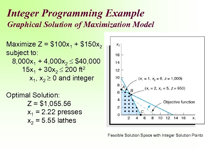
Integer Programming Example Graphical Solution of Maximization Model Maximize Z = $100 x 1 + $150 x 2 subject to: 8, 000 x 1 + 4, 000 x 2 $40, 000 15 x 1 + 30 x 2 200 ft 2 x 1, x 2 0 and integer Optimal Solution: Z = $1, 055. 56 x 1 = 2. 22 presses x 2 = 5. 55 lathes Feasible Solution Space with Integer Solution Points
Why not enumerate all the feasible integer points and select the best one? Enumerating all the integer solutions is impractical because of the large number of feasible integer points. Is rounding ever done? Yes, particularly if: - The values of the positive decision variables are relatively large, and - The values of the objective function coefficients relatively small.

General Integer Variables: Pure Integer Programming Models

Pure Integer Programming Example 1: Harrison Electric Company (1 of 8) • Produces two expensive products popular with renovators of historic old homes: – Ornate chandeliers (C) and – Old-fashioned ceiling fans (F). • Two-step production process: – Wiring ( 2 hours per chandelier and 3 hours per ceiling fan). – Final assembly time (6 hours per chandelier and 5 hours per fan).

Pure Integer Programming Example 1: Harrison Electric Company (2 of 8) • Production capability this period: – 12 hours of wiring time available and – 30 hours of final assembly time available. • Profits: – Chandelier profit $600 / unit and – Fan profit $700 / unit.

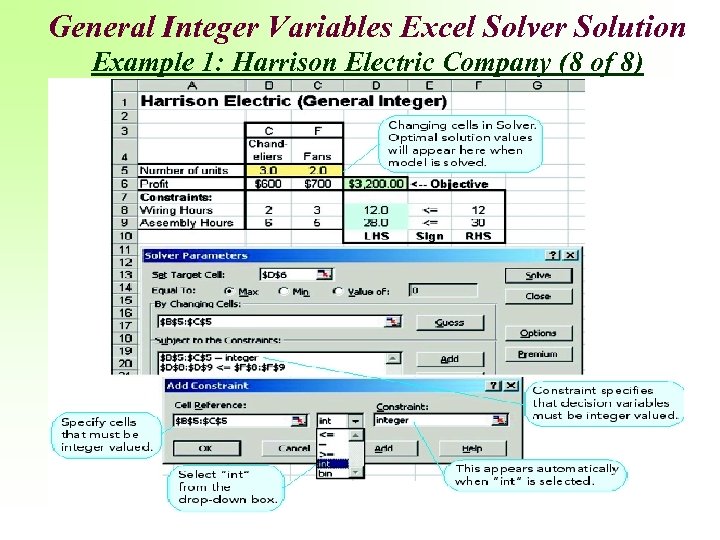
Pure Integer Programming Example 1: Harrison Electric Company (3 of 8) Objective: maximize profit = $600 C + $700 F subject to 2 C + 3 F <= 12 (wiring hours) 6 C + 5 F <= 30 (assembly hours) C, F >= 0 and integer where C = number of chandeliers to be produced F = number of ceiling fans to be produced
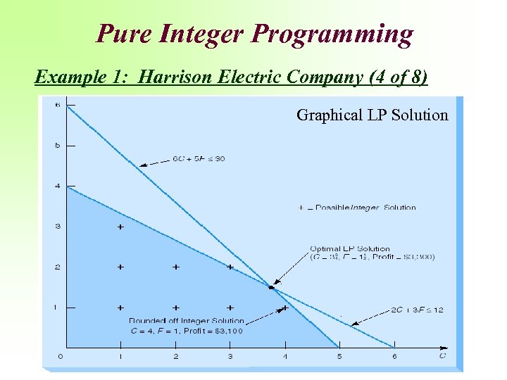
Pure Integer Programming Example 1: Harrison Electric Company (4 of 8) Graphical LP Solution

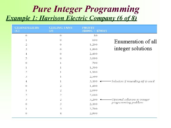
Pure Integer Programming Example 1: Harrison Electric Company (5 of 8) • Shaded region 1 shows feasible region for LP problem. • Optimal corner point solution: C = 3. 75 chandeliers and F = 1. 5 ceiling fans. • Profit of $3, 300 during production period. • But, we need to produce and sell integer values of the products. • The table shows all possible integer solutions for this problem.
Pure Integer Programming Example 1: Harrison Electric Company (6 of 8) Enumeration of all integer solutions

Pure Integer Programming Example 1: Harrison Electric Company (7 of 8) • Table lists the entire set of integer-valued solutions for problem. • By inspecting the right-hand column, optimal integer solution is: C = 3 chandeliers, F = 2 ceiling fans. • Total profit = $3, 200. • The rounded off solution: C = 4 F = 1 Total profit = $3, 100.
General Integer Variables Excel Solver Solution Example 1: Harrison Electric Company (8 of 8)
Solver Options
Premium Solver for Education

Pure Integer Programming Example 2: Boxcar Burger Restaurants (1 of 4) Boxcar Burger is a new chain of fast-food establishments. Boxcar is planning expansion in the downtown and suburban areas. Management would like to determine how many restaurants to open in each area in order to maximize net weekly profit.
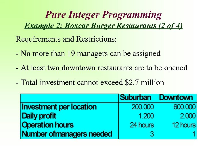
Pure Integer Programming Example 2: Boxcar Burger Restaurants (2 of 4) Requirements and Restrictions: - No more than 19 managers can be assigned - At least two downtown restaurants are to be opened - Total investment cannot exceed $2. 7 million
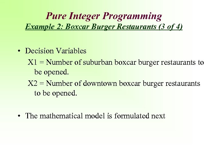
Pure Integer Programming Example 2: Boxcar Burger Restaurants (3 of 4) • Decision Variables X 1 = Number of suburban boxcar burger restaurants to be opened. X 2 = Number of downtown boxcar burger restaurants to be opened. • The mathematical model is formulated next
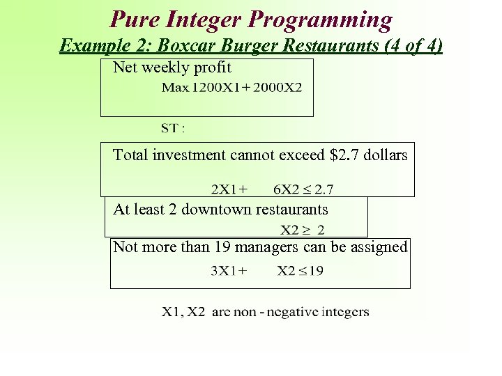
Pure Integer Programming Example 2: Boxcar Burger Restaurants (4 of 4) Net weekly profit Total investment cannot exceed $2. 7 dollars At least 2 downtown restaurants Not more than 19 managers can be assigned
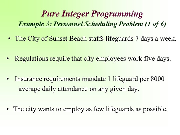
Pure Integer Programming Example 3: Personnel Scheduling Problem (1 of 6) • The City of Sunset Beach staffs lifeguards 7 days a week. • Regulations require that city employees work five days. • Insurance requirements mandate 1 lifeguard per 8000 average daily attendance on any given day. • The city wants to employ as few lifeguards as possible.
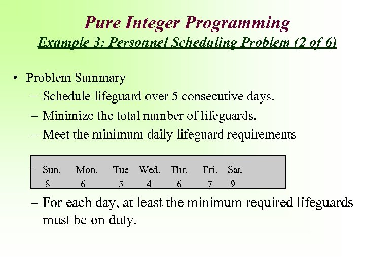
Pure Integer Programming Example 3: Personnel Scheduling Problem (2 of 6) • Problem Summary – Schedule lifeguard over 5 consecutive days. – Minimize the total number of lifeguards. – Meet the minimum daily lifeguard requirements – Sun. Mon. Tue Wed. Thr. Fri. Sat. 8 6 5 4 6 7 9 – For each day, at least the minimum required lifeguards must be on duty.
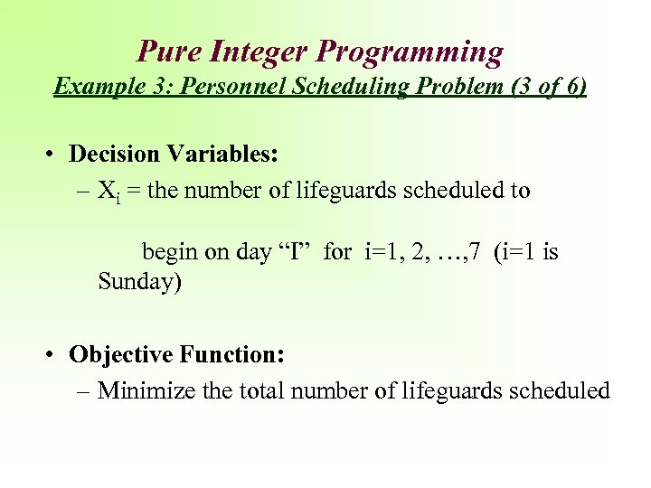
Pure Integer Programming Example 3: Personnel Scheduling Problem (3 of 6) • Decision Variables: – Xi = the number of lifeguards scheduled to begin on day “I” for i=1, 2, …, 7 (i=1 is Sunday) • Objective Function: – Minimize the total number of lifeguards scheduled
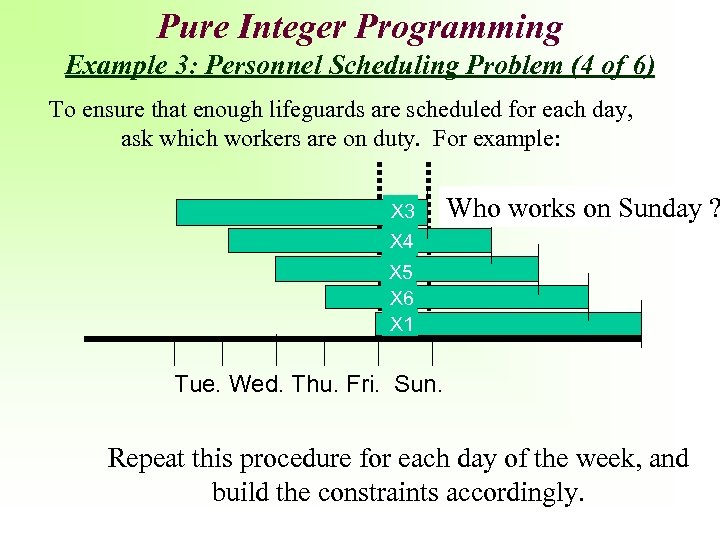
Pure Integer Programming Example 3: Personnel Scheduling Problem (4 of 6) To ensure that enough lifeguards are scheduled for each day, ask which workers are on duty. For example: X 3 X 4 Who works on Sunday ? X 5 X 6 X 1 Tue. Wed. Thu. Fri. Sun. Repeat this procedure for each day of the week, and build the constraints accordingly.
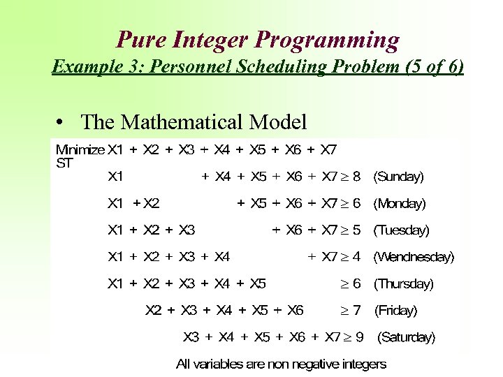
Pure Integer Programming Example 3: Personnel Scheduling Problem (5 of 6) • The Mathematical Model
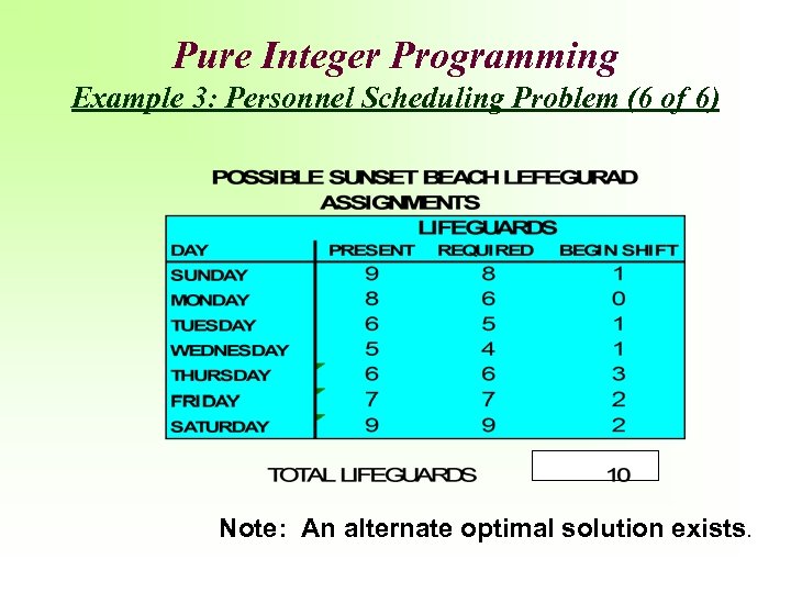
Pure Integer Programming Example 3: Personnel Scheduling Problem (6 of 6) Note: An alternate optimal solution exists.
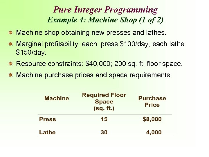
Pure Integer Programming Example 4: Machine Shop (1 of 2) Machine shop obtaining new presses and lathes. Marginal profitability: each press $100/day; each lathe $150/day. Resource constraints: $40, 000; 200 sq. ft. floor space. Machine purchase prices and space requirements:
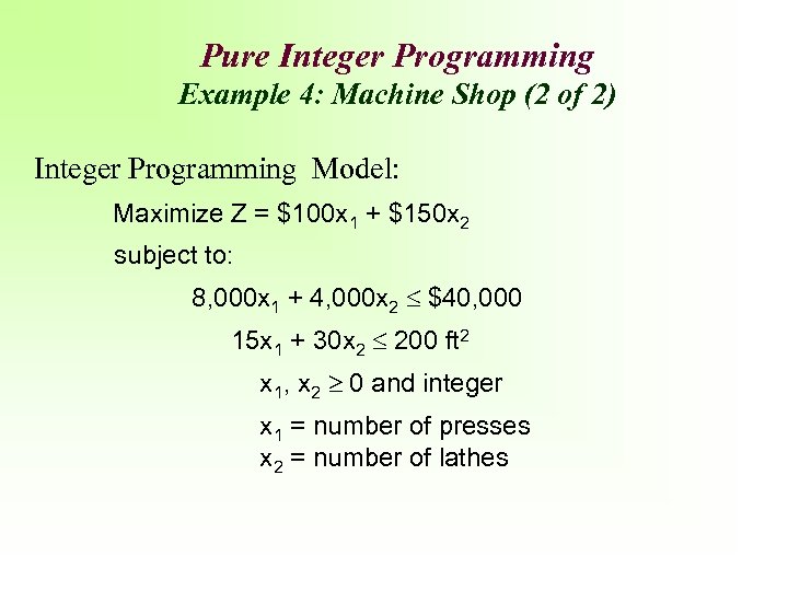
Pure Integer Programming Example 4: Machine Shop (2 of 2) Integer Programming Model: Maximize Z = $100 x 1 + $150 x 2 subject to: 8, 000 x 1 + 4, 000 x 2 $40, 000 15 x 1 + 30 x 2 200 ft 2 x 1, x 2 0 and integer x 1 = number of presses x 2 = number of lathes
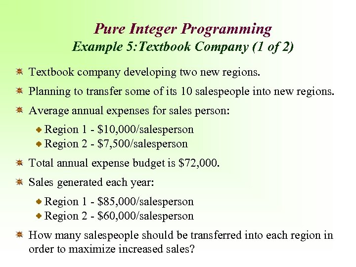
Pure Integer Programming Example 5: Textbook Company (1 of 2) Textbook company developing two new regions. Planning to transfer some of its 10 salespeople into new regions. Average annual expenses for sales person: Region 1 - $10, 000/salesperson Region 2 - $7, 500/salesperson Total annual expense budget is $72, 000. Sales generated each year: Region 1 - $85, 000/salesperson Region 2 - $60, 000/salesperson How many salespeople should be transferred into each region in order to maximize increased sales?
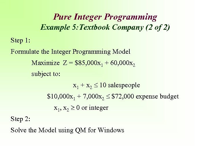
Pure Integer Programming Example 5: Textbook Company (2 of 2) Step 1: Formulate the Integer Programming Model Maximize Z = $85, 000 x 1 + 60, 000 x 2 subject to: x 1 + x 2 10 salespeople $10, 000 x 1 + 7, 000 x 2 $72, 000 expense budget x 1, x 2 0 or integer Step 2: Solve the Model using QM for Windows

Sensitivity in ILP • In ILP models, there is no pattern to the disjoint effects of changes to the objective function and right hand side coefficients. • When changes occur, they occur in big ”steps, ” rather than the smooth, marginal fashion experienced in linear programming. • Therefore, sensitivity analysis for integer models must be made by re-solving the problem, a very timeconsuming process.

General Integer Variables: Mixed Integer Programming Models
General Integer Variable (IP): Mixed Integer Programming • A mixed integer linear programming model is one in which some, but not all, the variables are restricted integers. • The Shelly Mednick Investment Problem illustrates this situation

Mixed Integer Linear Programming Example 1: Shelly Mednick Investment Problem (1 of 3) • Shelley Mednick has decided to give the stock market a try. • She will invest in – TCS, a communication company stock, and or, – MFI, a mutual fund. • Shelley is a cautious investor. She sets limits on the level of investments, and a modest goal for gain for the year.
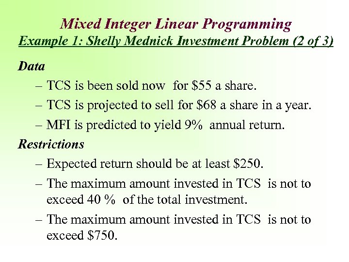
Mixed Integer Linear Programming Example 1: Shelly Mednick Investment Problem (2 of 3) Data – TCS is been sold now for $55 a share. – TCS is projected to sell for $68 a share in a year. – MFI is predicted to yield 9% annual return. Restrictions – Expected return should be at least $250. – The maximum amount invested in TCS is not to exceed 40 % of the total investment. – The maximum amount invested in TCS is not to exceed $750.
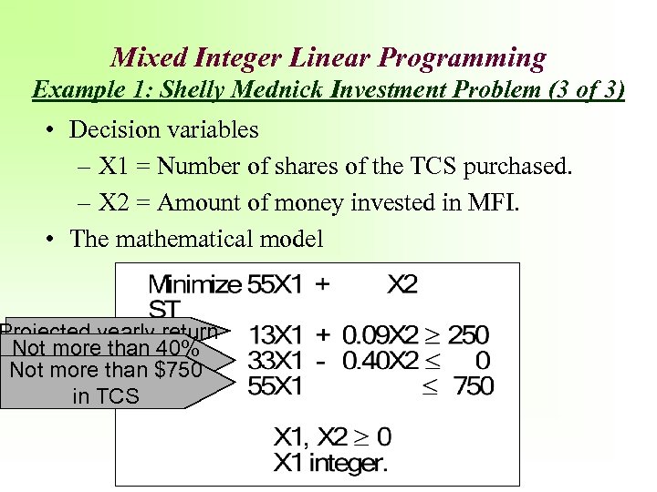
Mixed Integer Linear Programming Example 1: Shelly Mednick Investment Problem (3 of 3) • Decision variables – X 1 = Number of shares of the TCS purchased. – X 2 = Amount of money invested in MFI. • The mathematical model Projected yearly return Not more than 40% Not more. TCS $750 in than in TCS
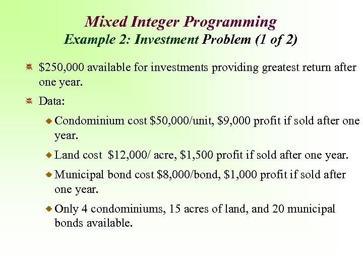
Mixed Integer Programming Example 2: Investment Problem (1 of 2) $250, 000 available for investments providing greatest return after one year. Data: Condominium cost $50, 000/unit, $9, 000 profit if sold after one year. Land cost $12, 000/ acre, $1, 500 profit if sold after one year. Municipal bond cost $8, 000/bond, $1, 000 profit if sold after one year. Only 4 condominiums, 15 acres of land, and 20 municipal bonds available.
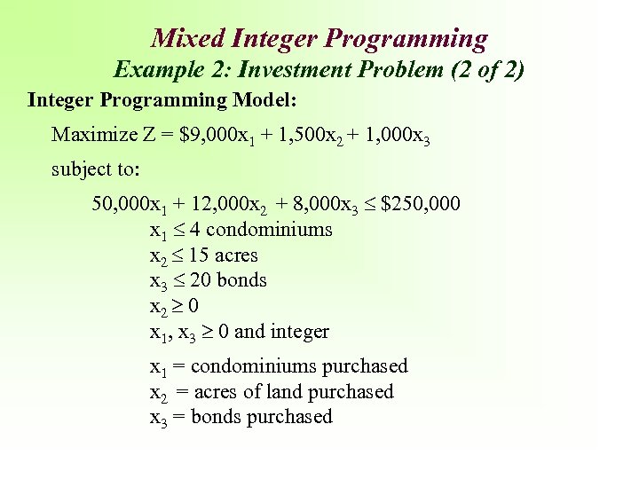
Mixed Integer Programming Example 2: Investment Problem (2 of 2) Integer Programming Model: Maximize Z = $9, 000 x 1 + 1, 500 x 2 + 1, 000 x 3 subject to: 50, 000 x 1 + 12, 000 x 2 + 8, 000 x 3 $250, 000 x 1 4 condominiums x 2 15 acres x 3 20 bonds x 2 0 x 1, x 3 0 and integer x 1 = condominiums purchased x 2 = acres of land purchased x 3 = bonds purchased

Models with Binary Variables
Models With Binary Variables Binary variables restricted to values of 0 or 1. • Model explicitly specifies that variables are binary. • Typical examples include decisions such as: – Introducing new product (introduce it or not), – Building new facility (build it or not), – Selecting team (select a specific individual or not), and – Investing in projects (invest in a specific project or not).
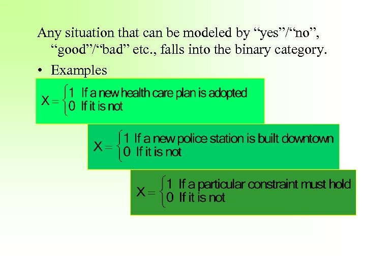
Any situation that can be modeled by “yes”/“no”, “good”/“bad” etc. , falls into the binary category. • Examples

Pure Binary Integer Programming Models

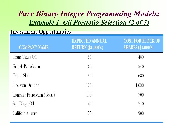
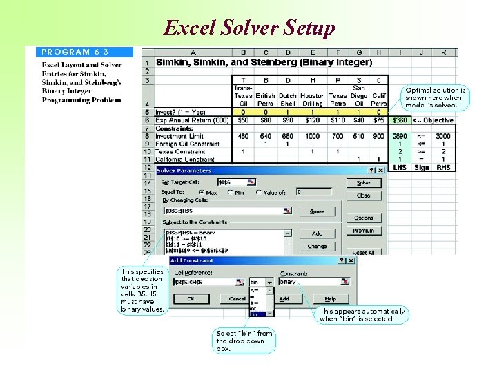
Pure Binary Integer Programming Models: Example 1: Oil Portfolio Selection (1 of 7) Firm specializes in recommending oil stock portfolios. • At least two Texas oil firms must be in portfolio. • No more than one investment can be made in foreign oil. • Exactly one of two California oil stocks must be purchased. • If British Petroleum stock is included in portfolio, then Texas-Trans Oil stock must also be included in portfolio. • Client has $3 million available for investments and insists on purchasing large blocks of shares of each company for investment. • Objective is to maximize annual return on investment.
Pure Binary Integer Programming Models: Example 1. Oil Portfolio Selection (2 of 7) Investment Opportunities

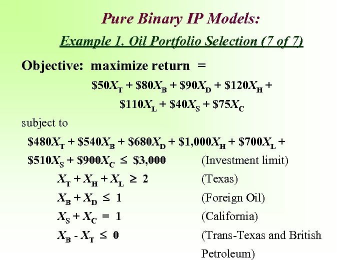
Pure Binary (0, 1) IP Models: Example 1. Oil Portfolio Selection (3 of 7) Objective: maximize return on investment = $50 XT + $80 XB + $90 XD + $120 XH + $110 XL + $40 XS + $75 XC Binary variable defined as: Xi = 1 if large block of shares in company i is purchased = 0 if large block of shares in company i is not purchased where i = T (for Trans-Texas Oil), B (for British Petroleum), D (for Dutch Shell), H (for Houston Drilling), L (for Lonestar Petroleum), S (for San Diego Oil), or C (for California Petro).
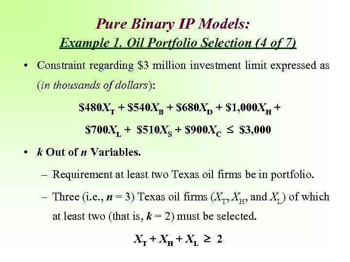
Pure Binary IP Models: Example 1. Oil Portfolio Selection (4 of 7) • Constraint regarding $3 million investment limit expressed as (in thousands of dollars): $480 XT + $540 XB + $680 XD + $1, 000 XH + $700 XL + $510 XS + $900 XC $3, 000 • k Out of n Variables. – Requirement at least two Texas oil firms be in portfolio. – Three (i. e. , n = 3) Texas oil firms (XT, XH, and XL) of which at least two (that is, k = 2) must be selected. XT + XH + XL 2
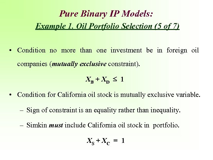
Pure Binary IP Models: Example 1. Oil Portfolio Selection (5 of 7) • Condition no more than one investment be in foreign oil companies (mutually exclusive constraint). XB + XD 1 • Condition for California oil stock is mutually exclusive variable. – Sign of constraint is an equality rather than inequality. – Simkin must include California oil stock in portfolio. XS + XC = 1
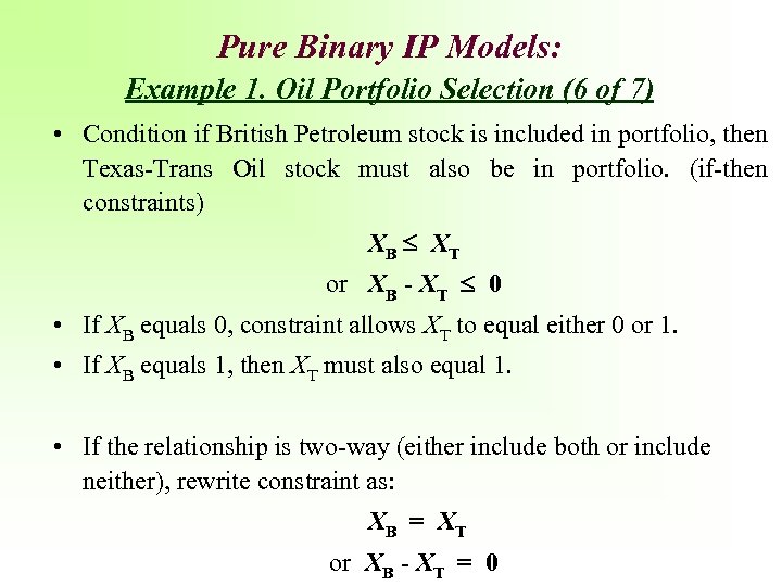
Pure Binary IP Models: Example 1. Oil Portfolio Selection (6 of 7) • Condition if British Petroleum stock is included in portfolio, then Texas-Trans Oil stock must also be in portfolio. (if-then constraints) XB XT or XB - XT 0 • If XB equals 0, constraint allows XT to equal either 0 or 1. • If XB equals 1, then XT must also equal 1. • If the relationship is two-way (either include both or include neither), rewrite constraint as: XB = XT or XB - XT = 0
Pure Binary IP Models: Example 1. Oil Portfolio Selection (7 of 7) Objective: maximize return = $50 XT + $80 XB + $90 XD + $120 XH + $110 XL + $40 XS + $75 XC subject to $480 XT + $540 XB + $680 XD + $1, 000 XH + $700 XL + $510 XS + $900 XC $3, 000 (Investment limit) XT + XH + XL 2 (Texas) XB + XD 1 (Foreign Oil) XS + XC = 1 (California) XB - XT 0 (Trans-Texas and British Petroleum)
Excel Solver Setup
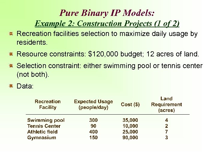
Pure Binary IP Models: Example 2: Construction Projects (1 of 2) Recreation facilities selection to maximize daily usage by residents. Resource constraints: $120, 000 budget; 12 acres of land. Selection constraint: either swimming pool or tennis center (not both). Data:
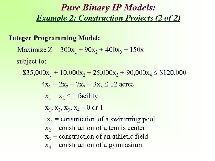
Pure Binary IP Models: Example 2: Construction Projects (2 of 2) Integer Programming Model: Maximize Z = 300 x 1 + 90 x 2 + 400 x 3 + 150 x subject to: $35, 000 x 1 + 10, 000 x 2 + 25, 000 x 3 + 90, 000 x 4 $120, 000 4 x 1 + 2 x 2 + 7 x 3 + 3 x 3 12 acres x 1 + x 2 1 facility x 1, x 2, x 3, x 4 = 0 or 1 x 1 = construction of a swimming pool x 2 = construction of a tennis center x 3 = construction of an athletic field x 4 = construction of a gymnasium
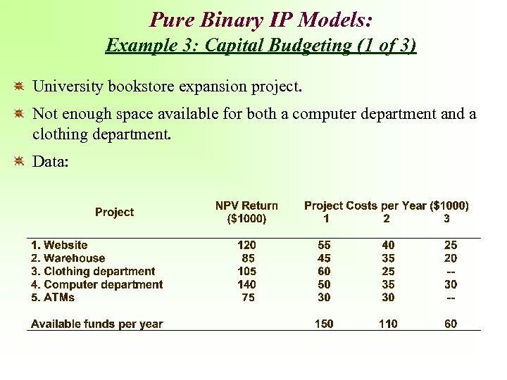
Pure Binary IP Models: Example 3: Capital Budgeting (1 of 3) University bookstore expansion project. Not enough space available for both a computer department and a clothing department. Data:
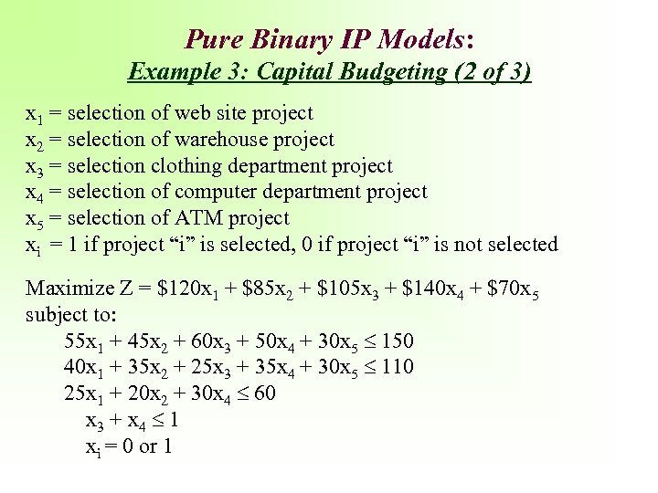
Pure Binary IP Models: Example 3: Capital Budgeting (2 of 3) x 1 = selection of web site project x 2 = selection of warehouse project x 3 = selection clothing department project x 4 = selection of computer department project x 5 = selection of ATM project xi = 1 if project “i” is selected, 0 if project “i” is not selected Maximize Z = $120 x 1 + $85 x 2 + $105 x 3 + $140 x 4 + $70 x 5 subject to: 55 x 1 + 45 x 2 + 60 x 3 + 50 x 4 + 30 x 5 150 40 x 1 + 35 x 2 + 25 x 3 + 35 x 4 + 30 x 5 110 25 x 1 + 20 x 2 + 30 x 4 60 x 3 + x 4 1 xi = 0 or 1
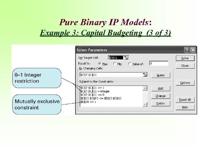
Pure Binary IP Models: Example 3: Capital Budgeting (3 of 3)
Pure Binary IP Models Example 4: Salem City Council (1 of 6) • The Salem City Council must choose projects to fund, such that public support is maximized • Relevant data covers constraints and concerns the City Council has, such as: – Estimated costs of each project. – Estimated number of permanent new jobs a project can create. – Questionnaire point tallies regarding the 9 project ranking.
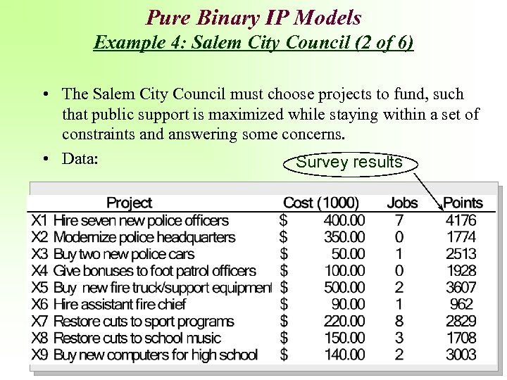
Pure Binary IP Models Example 4: Salem City Council (2 of 6) • The Salem City Council must choose projects to fund, such that public support is maximized while staying within a set of constraints and answering some concerns. • Data: Survey results
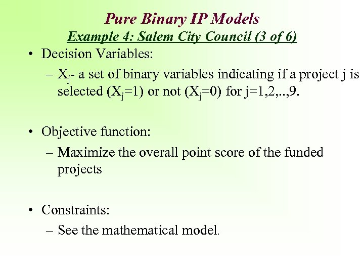
Pure Binary IP Models Example 4: Salem City Council (3 of 6) • Decision Variables: – Xj- a set of binary variables indicating if a project j is selected (Xj=1) or not (Xj=0) for j=1, 2, . . , 9. • Objective function: – Maximize the overall point score of the funded projects • Constraints: – See the mathematical model.
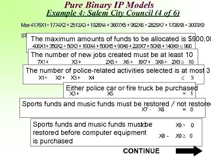
Pure Binary IP Models Example 4: Salem City Council (4 of 6) The maximum amounts of funds to be allocated is $900, 00 The number of new jobs created must be at least 10 The number of police-related activities selected is at most 3 Either police car or fire truck be purchased Sports funds and music funds must be restored / not restored Sports funds and music funds must be restored before computer equipment is purchased CONTINUE
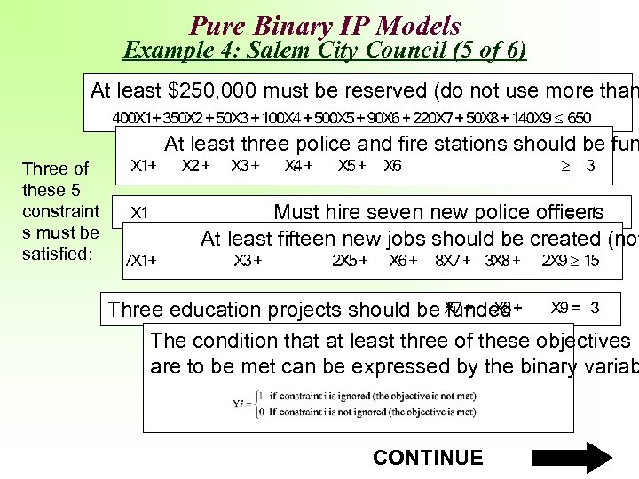
Pure Binary IP Models Example 4: Salem City Council (5 of 6) At least $250, 000 must be reserved (do not use more than At least three police and fire stations should be fun Three of these 5 constraint s must be satisfied: Must hire seven new police officers At least fifteen new jobs should be created (not Three education projects should be funded The condition that at least three of these objectives are to be met can be expressed by the binary variab CONTINUE
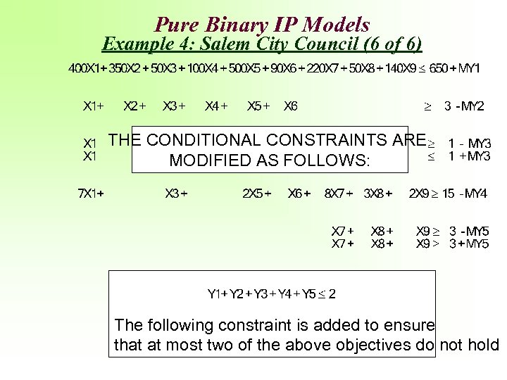
Pure Binary IP Models Example 4: Salem City Council (6 of 6) THE CONDITIONAL CONSTRAINTS ARE MODIFIED AS FOLLOWS: The following constraint is added to ensure that at most two of the above objectives do not hold

Mixed Binary Integer Programming Models
Mixed Binary Integer Programming Models – Fixed Charge Problems • Fixed costs may include costs to set up machines for production run or construction costs to build new facility. – Fixed costs are independent of volume of production. – Incurred whenever decision to go ahead with project is taken. • Linear programming does not include fixed costs in its cost considerations. It assumes these costs as costs that cannot be avoided. However, this may be incorrect.
Problems involving fixed and variable costs are mixed integer programming models or fixed-charge problems. • Binary variables are used for fixed costs. • Ensures whenever a decision variable associated with variable cost is non-zero, the binary variable associated with fixed cost takes on a value of 1 (i. e. , fixed cost is also incurred).
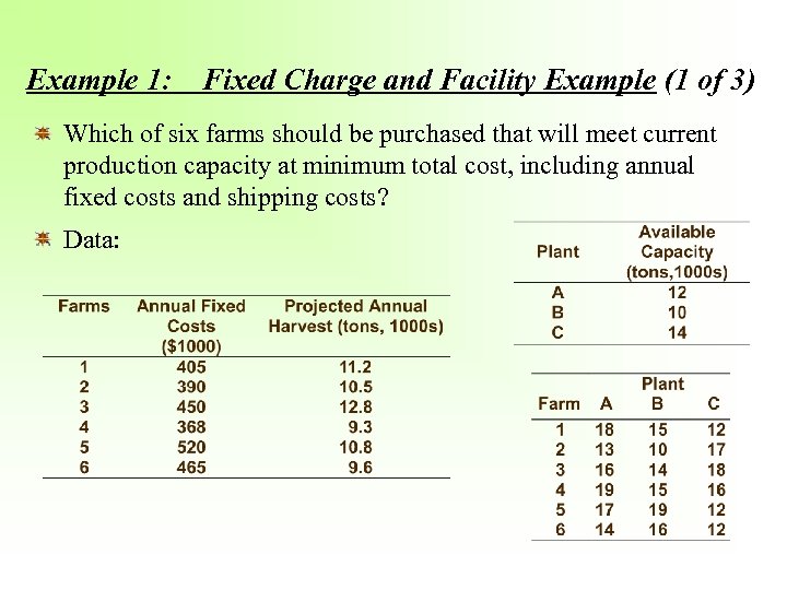
Example 1: Fixed Charge and Facility Example (1 of 3) Which of six farms should be purchased that will meet current production capacity at minimum total cost, including annual fixed costs and shipping costs? Data:
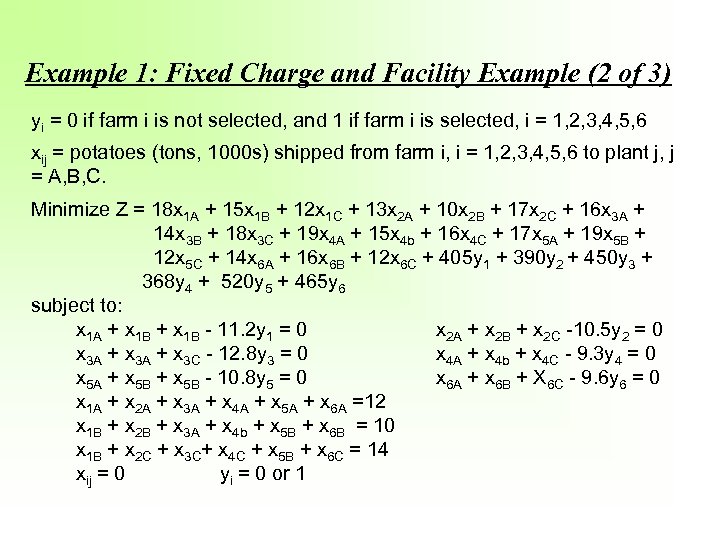
Example 1: Fixed Charge and Facility Example (2 of 3) yi = 0 if farm i is not selected, and 1 if farm i is selected, i = 1, 2, 3, 4, 5, 6 xij = potatoes (tons, 1000 s) shipped from farm i, i = 1, 2, 3, 4, 5, 6 to plant j, j = A, B, C. Minimize Z = 18 x 1 A + 15 x 1 B + 12 x 1 C + 13 x 2 A + 10 x 2 B + 17 x 2 C + 16 x 3 A + 14 x 3 B + 18 x 3 C + 19 x 4 A + 15 x 4 b + 16 x 4 C + 17 x 5 A + 19 x 5 B + 12 x 5 C + 14 x 6 A + 16 x 6 B + 12 x 6 C + 405 y 1 + 390 y 2 + 450 y 3 + 368 y 4 + 520 y 5 + 465 y 6 subject to: x 1 A + x 1 B - 11. 2 y 1 = 0 x 2 A + x 2 B + x 2 C -10. 5 y 2 = 0 x 3 A + x 3 C - 12. 8 y 3 = 0 x 4 A + x 4 b + x 4 C - 9. 3 y 4 = 0 x 5 A + x 5 B - 10. 8 y 5 = 0 x 6 A + x 6 B + X 6 C - 9. 6 y 6 = 0 x 1 A + x 2 A + x 3 A + x 4 A + x 5 A + x 6 A =12 x 1 B + x 2 B + x 3 A + x 4 b + x 5 B + x 6 B = 10 x 1 B + x 2 C + x 3 C+ x 4 C + x 5 B + x 6 C = 14 xij = 0 yi = 0 or 1
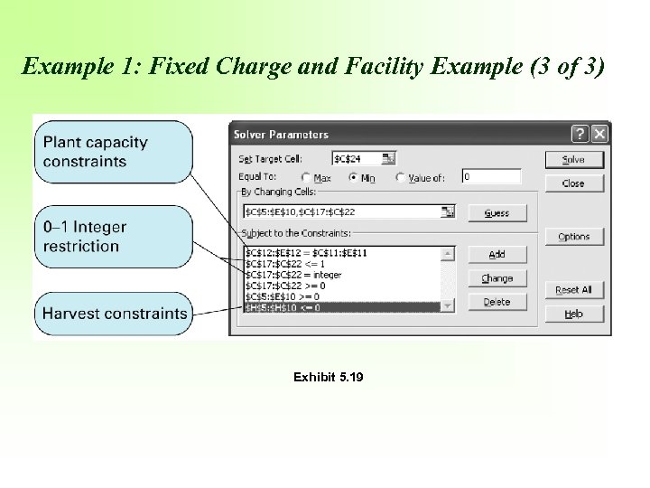
Example 1: Fixed Charge and Facility Example (3 of 3) Exhibit 5. 19
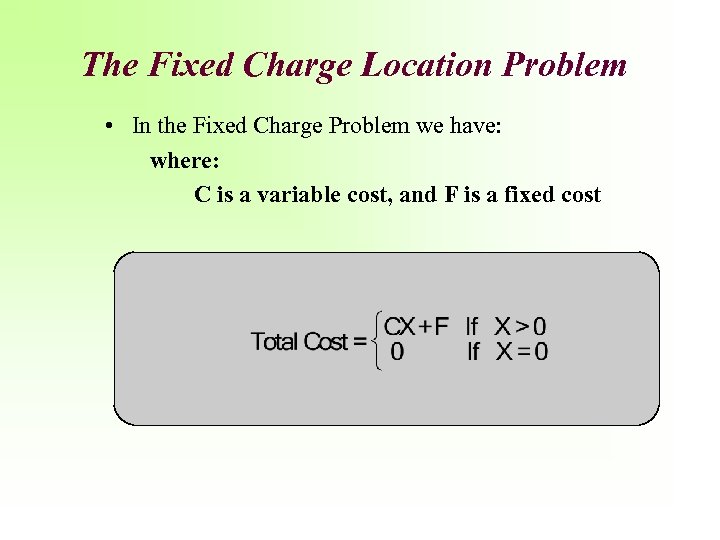
The Fixed Charge Location Problem • In the Fixed Charge Problem we have: where: C is a variable cost, and F is a fixed cost

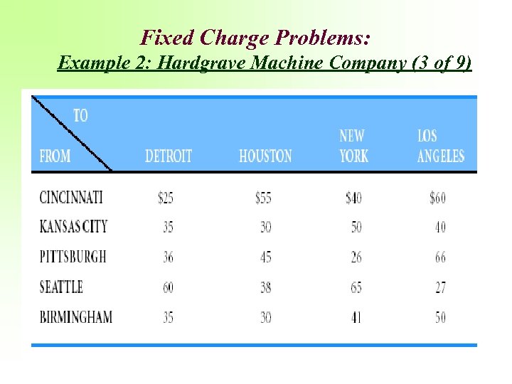
Fixed Charge Problems: Example 2: Hardgrave Machine Company –Location (1 of 9) • Produces computer components at its plants in Cincinnati and Pittsburgh. – Plants are not able to keep up with demand for orders at warehouses in Detroit, Houston, New York, and Los Angeles. – Firm is to build a new plant to expand its productive capacity. – Sites being considered are Seattle, Washington and Birmingham. • Table presents - – Production costs and capacities for existing plants and demand at each warehouse. – Estimated production costs of new (proposed) plants. • Transportation costs from plants to warehouses are also summarized in the Table
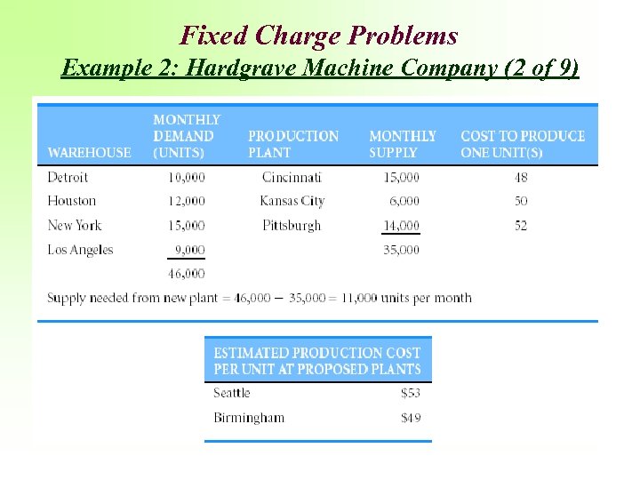
Fixed Charge Problems Example 2: Hardgrave Machine Company (2 of 9)
Fixed Charge Problems: Example 2: Hardgrave Machine Company (3 of 9)

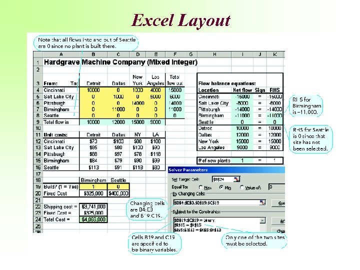
Fixed Charge Problems: Example 2: Hardgrave Machine Company (4 of 9) • Monthly fixed costs are $400, 000 in Seattle and $325, 000 in Birmingham • Which new location will yield lowest cost in combination with existing plants and warehouses? • Unit cost of shipping from each plant to warehouse is found by adding shipping costs to production costs • Solution must consider monthly fixed costs of operating new facility.

Fixed Charge Problems Example 2: Hardgrave Machine Company (5 of 9) • Use binary variables for each of the two locations. YS = 1 if Seattle selected as new plant. = 0 otherwise. YB = 1 if Birmingham is selected as new plant. = 0 otherwise. • Use binary variables for representative quantities. Xij = # of units shipped from plant i to warehouse j where i = C (Cincinnati), K (Kansas City), P ( Pittsburgh), S ( Seattle), or B (Birmingham) j = D (Detroit), H (Houston), N (New York), or L (Los Angeles)
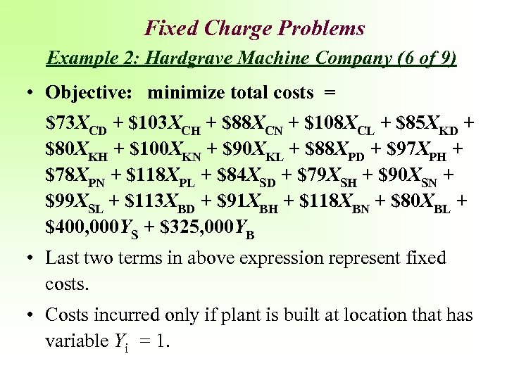
Fixed Charge Problems Example 2: Hardgrave Machine Company (6 of 9) • Objective: minimize total costs = $73 XCD + $103 XCH + $88 XCN + $108 XCL + $85 XKD + $80 XKH + $100 XKN + $90 XKL + $88 XPD + $97 XPH + $78 XPN + $118 XPL + $84 XSD + $79 XSH + $90 XSN + $99 XSL + $113 XBD + $91 XBH + $118 XBN + $80 XBL + $400, 000 YS + $325, 000 YB • Last two terms in above expression represent fixed costs. • Costs incurred only if plant is built at location that has variable Yi = 1.

Fixed Charge Problems Example 2: Hardgrave Machine Company (7 of 9) • Flow balance constraints at plants and warehouses: Net flow = (Total flow in to node) - (Total flow out of node) • Flow balance constraints at existing plants (Cincinnati, Kansas City, and Pittsburgh) : (0) - (XCD + XCH + XCN + XCL) = -15, 000 (Cincinnati supply) (0) - (XKD + XKH + XKN + XKL) = -6, 000 (Kansas City supply) (0) - (XPD + XPH + XPN + XPL) = -14, 000 (Pittsburgh supply) • Flow balance constraint for new plant - account for the 0, 1 (Binary) YS and YB variables: (0) - (XSD + XSH + XSN + XSL) = -11, 000 YS (Seattle supply) (0) - (XBD + XBH + XBN + XBL) = -11, 000 YB (Birmingham supply)
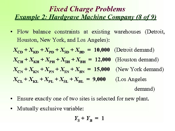
Fixed Charge Problems Example 2: Hardgrave Machine Company (8 of 9) • Flow balance constraints at existing warehouses (Detroit, Houston, New York, and Los Angeles): XCD + XKD + XPD + XSD + XBD = 10, 000 (Detroit demand) XCH + XKH + XPH + XSH + XBH = 12, 000 (Houston demand) XCN + XKN + XPN + XSN + XBN = 15, 000 (New York demand) XCL + XKL + XPL + XSL + XBL = 9, 000 (Los Angeles demand) • Ensure exactly one of two sites is selected for new plant. • Mutually exclusive variable: YS + YB = 1
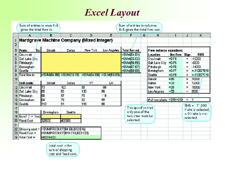
Excel Layout

Fixed Charge Problems Example 2: Hardgrave Machine Company (9 of 9) • Cost of shipping was $3, 704, 000 if new plant built at Seattle. • Cost was $3, 741, 000 if new plant built at Birmingham. • Including fixed costs, total costs would be: Seattle: $3, 704, 000 + $400, 000 = $4, 104, 000 Birmingham: $3, 741, 000 + $325, 000 = $4, 066, 000 • Select Birmingham as site for new plant.
Excel Layout

Globe Electronics, Inc. Two Different Problems, Two Different Models

Fixed Charge Problems Example 3. Globe Electronics, Inc. Data (1 of 5) • Globe Electronics, Inc. manufactures two styles of remote control cable boxes, G 50 and G 90. • Globe runs four production facilities and three distribution centers. • Each plant operates under unique conditions, thus has a different fixed operating cost, production costs, production rate, and production time available.
Fixed Charge Problems Example 3. Globe Electronics, Inc. Data (2 of 5) Demand has decreased, therefore, management is contemplating either: - working undercapacity at one or some of its plants or, - closing one or more of its facilities. So Management wishes to: – Develop an optimal distribution policy. – Determine which plant(s) to be 1) operated under capacity or closed (if any).
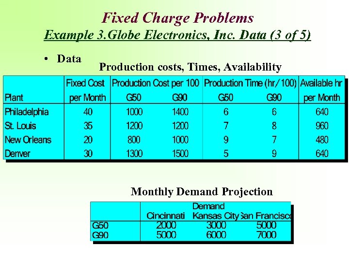
Fixed Charge Problems Example 3. Globe Electronics, Inc. Data (3 of 5) • Data Production costs, Times, Availability Monthly Demand Projection

Fixed Charge Problems Example 3. Globe Electronics, Inc. Data (4 of 5) – Transportation Costs per 100 units Cincinnati Philadelphia $200 Kansas City 300 St. Louis New Orleans Denver 100 200 300 100 200 100 San Francisco 500 400 300 100 – At least 70% of the demand in each distribution center must be satisfied. – Unit selling price • G 50 = $22; G 90 = $28.

Fixed Charge Problems Example 3. Globe Electronics, Inc. Dec. Vrbs. (5 of 5) • Decision Variables Xi = hundreds of G 50 s produced at plant i Zi = hundreds of G 90 s produced at plant i Xij = hundreds of G 50 s shipped from plant i to distribution center j Zij = hundreds of G 90 s shipped from plant i to distribution center j Location Identification

Globe Electronics Model No. 1: All The Plants Remain Operational
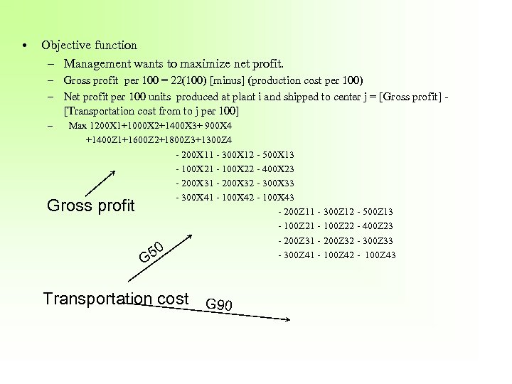
• Objective function – Management wants to maximize net profit. – Gross profit per 100 = 22(100) [minus] (production cost per 100) – Net profit per 100 units produced at plant i and shipped to center j = [Gross profit] [Transportation cost from to j per 100] – Max 1200 X 1+1000 X 2+1400 X 3+ 900 X 4 +1400 Z 1+1600 Z 2+1800 Z 3+1300 Z 4 - 200 X 11 - 300 X 12 - 500 X 13 - 100 X 21 - 100 X 22 - 400 X 23 - 200 X 31 - 200 X 32 - 300 X 33 - 300 X 41 - 100 X 42 - 100 X 43 - 200 Z 11 - 300 Z 12 - 500 Z 13 - 100 Z 21 - 100 Z 22 - 400 Z 23 - 200 Z 31 - 200 Z 32 - 300 Z 33 0 5 - 300 Z 41 - 100 Z 42 - 100 Z 43 Gross profit G Transportation cost G 90
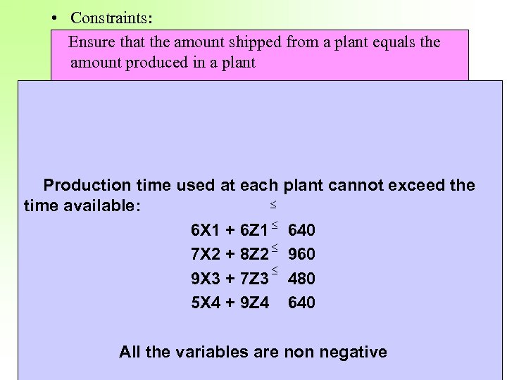
• Constraints: Ensure that the amount shipped from a plant equals the amount produced in a plant For G 50 For G 90 X 11 + X 12 + X 13 = X 1 X 21 + X 22 + X 23 = X 2 X 31 + X 32 + X 33 = X 3 X 41 + X 42 + X 43 = X 4 Z 11 + Z 12 + Z 13 = Z 1 Z 21 + Z 22 + Z 23 = Z 2 Z 31 + Z 32 + Z 33 = Z 3 Z 41 + Z 42 + Z 43 = Z 4 Production received byat each plant cannot the Amount time used a distribution center exceed time available: exceed its demand or G 50 6 X 1 + 6 Z 1 640 demand For be less than 70% of its For G 90 Z 11 X 11 + X 21 + X 31 + X 41 < 20 7 X 2 + 8 Z 2 960 + Z 21 +Z 31 + Z 41 < 50 X 11 + X 21 + X 31 + X 41 > 14 9 X 3 + 7 Z 3 480 Z 11 + Z 21 + Z 31 + Z 41 > X 12 + X 22 + X 32 + X 42 < 30 5 X 4 + 35 X 12 + X 22 + X 32 + X 42 > 21 9 Z 4 640 X 13 + X 23 + X 33 + X 43 < 50 X 13 + X 23 + X 33 + X 43 > 35 Z 12 + Z 22 + Z 32 + Z 42 < 60 All the variables are non negative Z 12 + Z 22 + Z 32 + Z 42 >
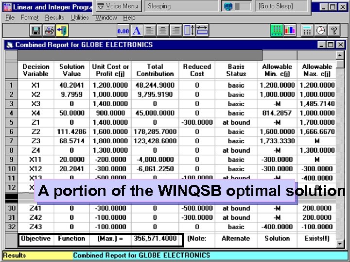
A portion of the WINQSB optimal solution
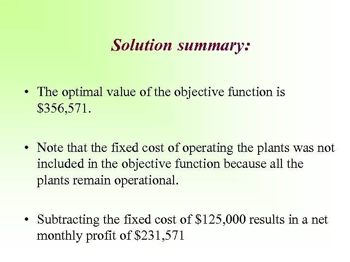
Solution summary: • The optimal value of the objective function is $356, 571. • Note that the fixed cost of operating the plants was not included in the objective function because all the plants remain operational. • Subtracting the fixed cost of $125, 000 results in a net monthly profit of $231, 571

Globe Electronics Model No. 2: The number of plants that remain operational is a decision variable
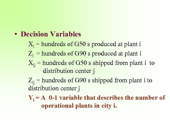
• Decision Variables Xi = hundreds of G 50 s produced at plant i Zi = hundreds of G 90 s produced at plant i Xij = hundreds of G 50 s shipped from plant i to distribution center j Zij = hundreds of G 90 s shipped from plant i to distribution center j Yi = A 0 -1 variable that describes the number of operational plants in city i.
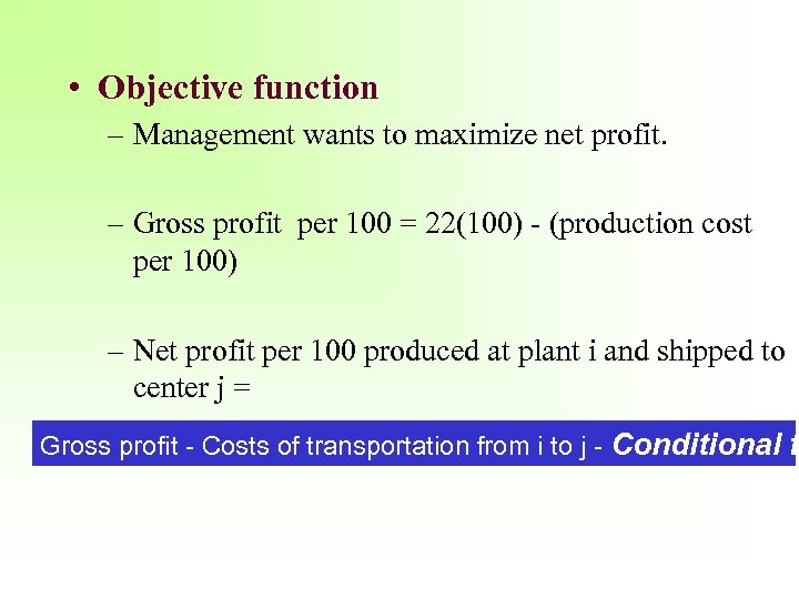
• Objective function – Management wants to maximize net profit. – Gross profit per 100 = 22(100) - (production cost per 100) – Net profit per 100 produced at plant i and shipped to center j = Gross profit - Costs of transportation from i to j - Conditional f
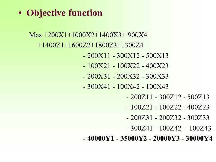
• Objective function Max 1200 X 1+1000 X 2+1400 X 3+ 900 X 4 +1400 Z 1+1600 Z 2+1800 Z 3+1300 Z 4 - 200 X 11 - 300 X 12 - 500 X 13 - 100 X 21 - 100 X 22 - 400 X 23 - 200 X 31 - 200 X 32 - 300 X 33 - 300 X 41 - 100 X 42 - 100 X 43 - 200 Z 11 - 300 Z 12 - 500 Z 13 - 100 Z 21 - 100 Z 22 - 400 Z 23 - 200 Z 31 - 200 Z 32 - 300 Z 33 - 300 Z 41 - 100 Z 42 - 100 Z 43 - 40000 Y 1 - 35000 Y 2 - 20000 Y 3 - 30000 Y 4
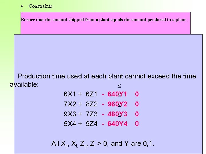
• Constraints: Ensure that the amount shipped from a plant equals the amount produced in a plant For G 50 For G 90 X 11 + X 12 + X 13 = X 1 X 21 + X 22 + X 23 = X 2 X 31 + X 32 + X 33 = X 3 X 41 + X 42 + X 43 = X 4 Z 11 + Z 12 + Z 13 = Z 1 Z 21 + Z 22 + Z 23 = Z 2 Z 31 + Z 32 + Z 33 = Z 3 Z 41 + Z 42 + Z 43 = Z 4 Amount received at a distribution center cannot Production time used by each plant cannot exceed the time exceed available: its demand or G 50 + 6 Z 1 -70% of its demand For be less than 640 Y 1 0 For G 90 6 X 1 X 11 + X 21 + X 31 + X 41 < 20 Z 11 + Z 21 +Z 31 + Z 41 < X 13 + X 23 + X 33 + X 43 < 50 X 13 + X 23 + X 33 + X 43 > Z 12 + Z 22 + Z 32 + Z 42 < 7 X 2 + 8 Z 2 - 960 Y 2 0 50 X 11 + X 21 + X 31 + X 41 > 14 9 X 3 + < 30 Z 11 0 X 12 + X 22 + X 32 + X 42 7 Z 3 - 480 Y 3 + Z 21 + Z 31 + Z 41 > 5 X 4 + > 21 35 X 12 + X 22 + X 32 + X 42 9 Z 4 - 640 Y 4 0 35 All Xij, Xi, Zij, Zi > 0, and 60 i are 0, 1. Y Z 12 + Z 22 + Z 32 + Z 42 >
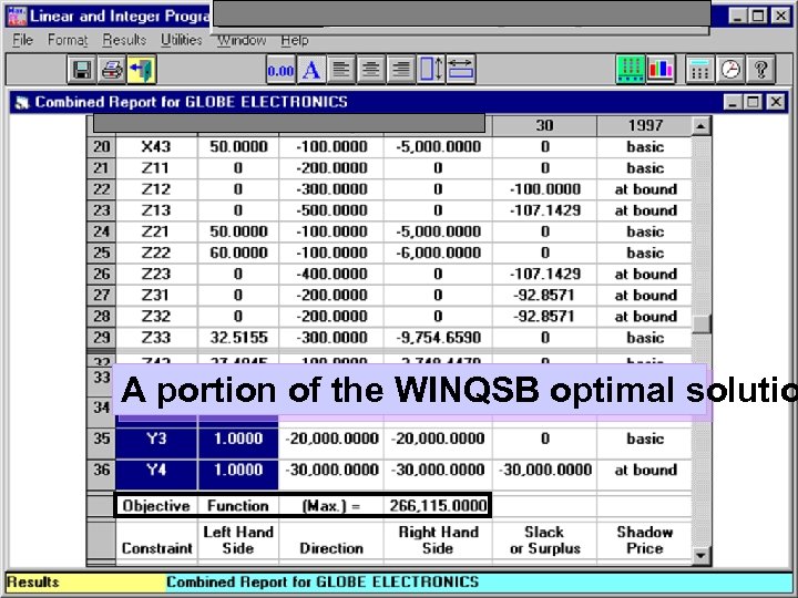
A portion of the WINQSB optimal solutio
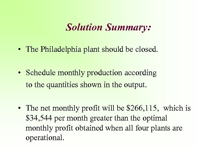
Solution Summary: • The Philadelphia plant should be closed. • Schedule monthly production according to the quantities shown in the output. • The net monthly profit will be $266, 115, which is $34, 544 per month greater than the optimal monthly profit obtained when all four plants are operational.
306796cb38611f7be5968e6b3e29816d.ppt