INSTRUMENTAL ANALYSIS CHEM 4811 CHAPTER 1 Dr au

INSTRUMENTAL ANALYSIS CHEM 4811 CHAPTER 1 Dr. au. Gustine ofori a. Gyeman assistant professor of chemistry Department of natural sciences clayton state university

CHAPTER 1 FUNDAMENTAL CONCEPTS

WHAT IS ANALYTICAL CHEMISTRY - The qualitative and quantitative characterization of matter - The scope is very wide and it is critical to our understanding of almost all scientific disciplines Characterization - The identification of chemical compounds or elements present in a sample (qualitative) - The determination of the amount of compound or element present in a sample (quantitative)

CHATACTERIZATION Qualitative Analysis - The identification of one or more chemical species present in a sample Quantitative Analysis - The determination of the exact amount of a chemical species present in a sample Chemical Species - Could be an element, ion or compound (organic or inorgnic)

CHATACTERIZATION Bulk Analysis - Characterization of the entire sample Example: determination of the elemental composition of a mixture (alloys) Surface Analysis - Characterization of the surface of a sample Example: finding the thickness of a thin layer on the surface of a solid material - Characterization may also include Structural Analysis and measurement of physical properties of materials

WET CHEMICAL ANALYSIS Volumetric Analysis - Analysis by volume Gravimetric Analysis - Analysis by mass - Wet analysis is time consuming and demands attention to detail Examples Acid-base titrations, redox titrations, complexometric titrations, precipitation reactions

WET CHEMICAL ANALYSIS Nondestructive Analysis - Useful when evidence needs to be preserved - Used to analyze samples without destroying them Examples Forensic analysis Paintings

INSTRUMENTAL ANALYSIS - Use of automated instruments in place of volumetric methods - Carried out by specially designed instruments which are controlled by computers - Samples are characterized by the interaction of electromagnetic radiation and matter - All the analytical steps (from sample preparation through data processing) are automated

INSTRUMENTAL ANALYSIS This course covers - The fundamentals of common analytical instruments - Measurements with these instruments - Interpretation of data obtained from the measurements - Communication of the meaning of the results

THE ANALYTICAL APPROACH - Problems continuously occur around the world in - Manufacturing industries - The environment - The health sector (medicine) etc. - The analytical chemist is the solution to these problems -The analytical chemist must understand the analytical approach uses, capabilities, and limitations of analytical techniques

THE ANALYTICAL APPROACH Analyte - A substance to be measured in a given sample Matrix - Everything else in the sample Interferences - Other compounds in the sample matrix that interfere with the measurement of the analyte

THE ANALYTICAL APPROACH Homogeneous Sample - Same chemical composition throughout (steel, sugar water, juice with no pulp, alcoholic beverages) Heterogeneous Sample - Composition varies from region to region within the sample (pudding with raisins, granola bars with peanuts) - Differences in composition may be visible or invisible to the human eye (most real samples are invisible) - Variation of composition may be random or segregated

THE ANALYTICAL APPROACH Analyze/Analysis - Applied to the sample under study Determine/Determination - Applied to the measurement of the analyte in the sample Multiple Samples - Identically prepared from another source Replicate Samples - Splits of sample from the same source

THE ANALYTICAL APPROACH General Steps in Chemical Analysis 1. Formulating the question or defining the problem - To be answered through chemical measurements 2. Designing the analytical method (selecting techniques) - Find appropriate analytical procedures 3. Sampling and sample storage - Select representative material to be analyzed 4. Sample preparation - Convert representative material into a suitable form for analysis

THE ANALYTICAL APPROACH General Steps in Chemical Analysis 5. Analysis (performing the measurement) - Measure the concentration of analyte in several identical portions 6. Assessing the data 7. Method validation 8. Documentation

DEFINING THE PROBLEM - Find out the information that needs to be known about a sample (or what procedure is being studied) - How accurate and precise the information must be - Whether qualitative or quantitative analysis or both is required - How much sample is available for study - Whether nondestructive analysis must be employed

DEFINING THE PROBLEM - Bulk analysis or analysis of certain parts is required - Sample is organic or inorganic - Sample a pure substance or a mixture - Homogeneous or heterogeneous sample - Chemical information or elemental information needed

DEFINING THE PROBLEM Qualitative Analysis - Provides information about what is present in the sample - If quantitative analysis is required, qualitative analysis is usually done first - Capabilities and limitations of analysis must be well understood

DEFINING THE PROBLEM Qualitative Analysis Qualitative Elemental Analysis - Used to identify elements present in a material - Can provide empirical formula of organic compounds (X-Ray Fluorescence, AAS) Qualitative Molecular Analysis - Used to identify molecules present in a material - Can be used to obtain molecular formula - Can be used to distinguish between isomers (NMR, IR, MS)

DEFINING THE PROBLEM Qualitative Analysis Empirical Formula - The simplest whole number ratios of atoms of each element present in a molecule Molecular Formula - Contains the total number of atoms of each element in a single molecule of the compound Isomers - Different structures with the same molecular formula (n-butane and iso-butane)

DEFINING THE PROBLEM Qualitative Analysis Enantiomers - Nonsuperimposable mirror-image isomers - Said to be chiral - Have the same IR, NMR, and MS - Mostly same physical properties (boiling-point, melting point, refractive index) - Chiral Chromatography can be used to distinguish between such optically active compounds (erythrose, glyceraldehyde)

DEFINING THE PROBLEM Qualitative Analysis Mixtures of Organic Compounds - Mixtures are usually separated before the individual components are identified - Separation techniques include GC LC HPLC CE

DEFINING THE PROBLEM Quantitative Analysis - The determination of the amount of analyte in a given sample - Often expressed in terms of concentrations Concentration - The quantity of analyte in a given volume or mass of sample Molarity = moles/liters, ppm = µg/g sample ppb = ng/g sample, ppt = pg/g sample Percent by mass [%(m/m)], Percent by volume [%(v/v)]

DEFINING THE PROBLEM Quantitative Analysis - Early methods include volumetric, gravimetric, and combustion analysis - Automated and extremely sensitive methods are being used today (GC, IR, HPLC, CE, XRD) - Require micron amounts and a few minutes Hyphenated techniques are used for qualitative and quantitative measurements of the components mixtures (GC-MS, LC-MS)

DESIGNING THE ANALYTICAL METHOD - Analytical procedure is designed after the problem has been defined Analyst must consider - Accuracy and precision - Amount of sample to be used - Cost analysis - Turnaround time (time between receipt of sample and delivery of results)

DESIGNING THE ANALYTICAL METHOD Green chemistry processes preferred for modern analytical procedures - The goal is to minimize waste and pollution - Use of less toxic or biodegradable solvents - Use of chemicals that can be recycled - Standard methods are available in literature (reproducible with known accuracy and precision)

DESIGNING THE ANALYTICAL METHOD - Do not waste time developing a method that already exists - Method of choice must be reliable and robust - Interferences must be evaluated Interference - Element or compound that respond directly to measurement to give false analyte signal - Signal may be enhanced or suppressed

DESIGNING THE ANALYTICAL METHOD Fundamental Features of Method - A blank must be analyzed - The blank is usually the pure solvent used for sample preparation - Used to identify and correct for interferences in the analysis - Analyst uses blank to set baseline Reagent blank: contains all the reagents used to prepare the sample Matrix blank: similar in chemical composition to the sample but without the analyte

DESIGNING THE ANALYTICAL METHOD Fundamental Features of Method - Methods require calibration standards (except coulometry) - Used to establish relationship between analytical signal being measured and the concentration of analyte - This relationship (known as the calibration curve) is used to determine the concentration of unknown analyte in samples

DESIGNING THE ANALYTICAL METHOD Fundamental Features of Method - Reference (check) standards are required - Standards of known composition with known concentration of analyte - Run as a sample to confirm that the calibration is correct - Used to access the precision and accuracy of the analysis Government and private sources of reference standards are available (National Institute of Standards and Technology, NIST)

SAMPLING - The most important step is the collection of the sample of the material to be analyzed - Sample should be representative of the material - Sample should be properly taken to provide reliable characterization of the material - Sufficient amount must be taken for all analysis Representative Sample - Reflects the true value and distribution of analyte in the original material

SAMPLING Steps in Sampling Process - Gross representative sample is collected from the lot - Portions of gross sample is taken from various parts of material Sampling methods include - Long pile and alternate shovel (used for very large lots) - Cone and quarter Aliquot - Quantitative amount of a test portion of sample solution

SAMPLING - Care must be taken since collection tools and storage containers can contaminate samples - Make room for multiple test portions of sample for replicate analysis or analysis by more than one technique Samples may undergo - grinding - chopping - milling - cutting

SAMPLING Gas Samples - Generally considered homogeneous - Samples are stirred before portions are taken for analysis - Gas samples may be filtered if solid materials are present Grab samples - Samples taken at a single point in time Composite Samples - Samples taken over a period of time or from different locations

SAMPLING Gas Samples Scrubbing - Trapping an analyte out of the gas phase Examples - Passing air through activated charcoal to adsorb organic vapors - Bubbling gas samples through a solution to absorb the analyte Samples may be taken with - Gas-tight syringes - Ballons (volatile organic compounds may contaminate samples) - Plastic bags (volatile organic compounds may contaminate samples) - Glass containers (may adsorb gas components)

SAMPLING Liquid Samples - May be collected as grab samples or composite samples - Adequate stirring is necessary to obtain representative sample - Stirring may not be desired under certain conditions (analysis of oily layer on water) - Undesired solid materials are removed by filtration or centrifugation - Layers of immiscible liquids may be separated with the separatory funnel

SAMPLING Solid Samples - The most difficult to sample since least homogeneous compared to gases and liquids - Large amounts are difficult to stir - Must undergo size reduction (milling, drilling, crushing, etc. ) to homogenize sample - Adsorbed water is often removed by oven drying

SAMPLING Sample Storage - Samples are stored if cannot be analyzed immediately - Sample composition can be changed by interaction with container material, light, or air - Appropriate storage container and conditions must be chosen - Organic components must not be stored in plastic containers due to leaching - Glass containers may adsorb or release trace levels of ionic species

SAMPLING Sample Storage - Appropriate cleaning of containers is necessary - Containers for organic samples are washed in solvent - Containers for metal samples are soaked in acid and deionized water - Containers must be first filled with inert gas to displace air - Biological samples are usually kept in freezers - Samples that interact with light are stored in the dark

SAMPLING Sample Storage - Some samples require p. H adjustment - Some samples require addition of preservatives (EDTA added to blood samples) - Appropriate labeling is necessary - Computer based Laboratory Information Management Systems (LIMS) are used to label and track samples

SAMPLE PREPARATION - Make samples in the physical form required by the instrument - Make concentrations in the range required by the instrument - Free analytes from interfering substances - Solvent is usually water or organic

SAMPLE PREPARATION Type of sample preparation depends on - nature of sample - technique chosen - analyte to be measured - the problem to be solved Samples may be - dissolved in water (or other solvents) - pressed into pellets - cast into thin films - etc.

SAMPLE PREPARATION METHODS - Specific methods are discussed in later chapters Acid Dissolution and Digestion - Used for dissolving metals, alloys, ores, glass, ceramics - Used for dissolving trace elements in organic materials (food, plastics) - Concentrated acid is added to sample and then heated - Choice of acid depends on sample to be dissolved analyte Acids commonly used: HCl, HNO 3, H 2 SO 4 HF and HCl. O 4 require special care and supervision

SAMPLE PREPARATION METHODS Fusion (Molten Salt Fusion) - Heating a finely powdered solid sample with a finely powdered salt at high temperatures until mixture melts - Useful for the determination of silica-containing minerals, glass, ceramics, bones, carbides Salts (Fluxes) Usually Used Sodium carbonate, sodium tetraborate (borax), sodium peroxide, lithium metaborate

SAMPLE PREPARATION METHODS Dry Ashing and Combustion - Burning an organic material in air or oxygen - Organic components form CO 2 and H 2 O vapor leaving inorganic components behind as solid oxides - Cannot be used for the determination of mercury, arsenic, and cadmium

SAMPLE PREPARATION METHODS Extraction - Used for determining organic analytes - Makes use of solvents - Solvents are chosen based on polarity of analyte (like dissolves like) Common Solvents Hexane, xylene, methylene chloride

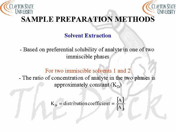SAMPLE PREPARATION METHODS Solvent Extraction - Based on preferential solubility of analyte in one of two immiscible phases For two immiscible solvents 1 and 2 - The ratio of concentration of analyte in the two phases is approximately constant (KD)

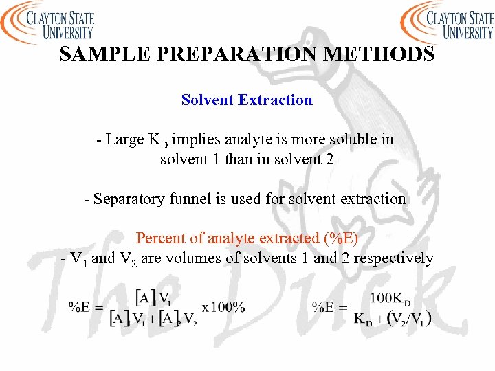SAMPLE PREPARATION METHODS Solvent Extraction - Large KD implies analyte is more soluble in solvent 1 than in solvent 2 - Separatory funnel is used for solvent extraction Percent of analyte extracted (%E) - V 1 and V 2 are volumes of solvents 1 and 2 respectively

SAMPLE PREPARATION METHODS Solvent Extraction - Multiple small extractions are more efficient than one large extraction - Extraction instruments are also available Examples Extraction of - pesticides, PCBs, petroluem hydrocarbons from water - fat from milk

SAMPLE PREPARATION METHODS Other Extraction Approaches Microwave Assisted Extraction - Heating with microwave energy during extraction Supercritical Fluid Extraction (SFE) - Use of supercritical CO 2 to dissolve organic compounds - Low cost, less toxic, ease of disposal Solid Phase Extraction (SPE) Solid Phase Microextraction (SPME) - The sample is a solid organic material - Extracted by passing sample through a bed of sorbent (extractant)

STATISTICS - Statistics are needed in designing the correct experiment Analyst must - select the required size of sample - select the number of samples - select the number of replicates - obtain the required accuracy and precision Analyst must also express uncertainty in measured values to - understand any associated limitations - know significant figures

STATISTICS Rules For Reporting Results Significant Figures = digits known with certainty + first uncertain digit - The last sig. fig. reflects the precision of the measurement - Report all sig. figs such that only the last figure is uncertain - Round off appropriately (round down, round up, round even)

STATISTICS Rules For Reporting Results - Report least sig. figs for multiplication and division of measurements (greatest number of absolute uncertainty) - Report least decimal places for addition and subtraction of measurements (greatest number of absolute uncertainty) - The characteristic of logarithm has no uncertainty - Does not affect the number of sig. figs. - Discrete objects have no uncertainty - Considered to have infinite number of sig. figs.

ACCURACY AND PRECISION - Accuracy is how close a measurement is to the true (accepted) value - True value is evaluated by analyzing known standard samples - Precision is how close replicate measurements on the sample are to each other - Precision is required for accuracy but does not guarantee accuracy - Results should be accurate and precise (reproducible, reliable, truly representative of sample)

ERRORS - Two principal types of errors - Determinate (systematic) and indeterminate (random) Determinate (Systematic) Errors - Caused by faults in procedure or instrument - Fault can be found out and corrected - Results in good precision but poor accuracy May be - constant (incorrect calibration of p. H meter or mass balance) - variable (change in volume due to temperature changes) - additive or multiplicative

ERRORS - Two principal types of errors - Determinate (systematic) and indeterminate (random) Examples of Determinate (Systematic) Errors - Uncalibrated or improperly calibrated mass balances - Improperly calibrated volumetric flasks and pipettes - Analyst error (misreading or inexperience) - Incorrect technique - Malfunctioning instrument (voltage fluctuations, alignment, etc) - Contaminated or impure or decomposed reagents - Interferences

ERRORS - Two principal types of errors - Determinate (systematic) and indeterminate (random) To Identify Determinate (Systematic) Errors - Use of standard methods with known accuracy and precision to analyze samples - Run several analysis of a reference analyte whose concentration is known and accepted - Run Standard Operating Procedures (SOPs)

ERRORS - Two principal types of errors - Determinate (systematic) and indeterminate (random) Indeterminate (Random) Errors - Sources cannot be identified, avoided, or corrected - Not constant (biased) Examples - Limitations of reading mass balances - Electrical noise in instruments

ERRORS - Random errors are always associated with measurements - No conclusion can be drawn with complete certainty - Scientists use statistics to accept conclusions that have high probability of being correct and to reject conclusions that have low probability of being correct - Random errors follow random distribution and analyzed using laws of probability - Statistics deals with only random errors - Systematic errors should be detected and eliminated

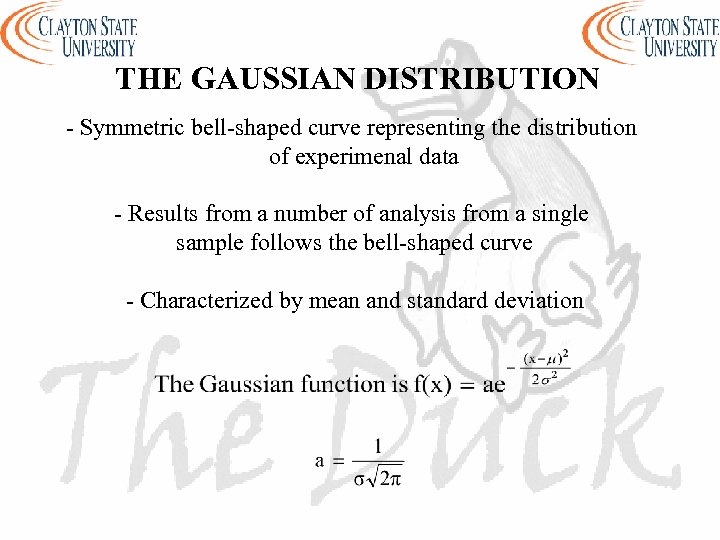THE GAUSSIAN DISTRIBUTION - Symmetric bell-shaped curve representing the distribution of experimenal data - Results from a number of analysis from a single sample follows the bell-shaped curve - Characterized by mean and standard deviation

THE GAUSSIAN DISTRIBUTION - a is the height of the curve’s peak - µ is the position of the center of the peak (the mean) - σ is a measure of the width of the curve (standard deviation) - T (or xt) is the accepted value - The larger the random error the broader the distribution - There is a difference between the values obtained from a finite number of measurements (N) and those obtained from infinite number of measurements

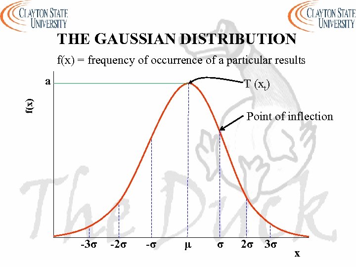THE GAUSSIAN DISTRIBUTION f(x) = frequency of occurrence of a particular results a f(x) T (xt) Point of inflection -3σ -2σ -σ μ σ 2σ 3σ x

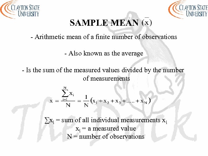SAMPLE MEAN - Arithmetic mean of a finite number of observations - Also known as the average - Is the sum of the measured values divided by the number of measurements ∑xi = sum of all individual measurements xi xi = a measured value N = number of observations

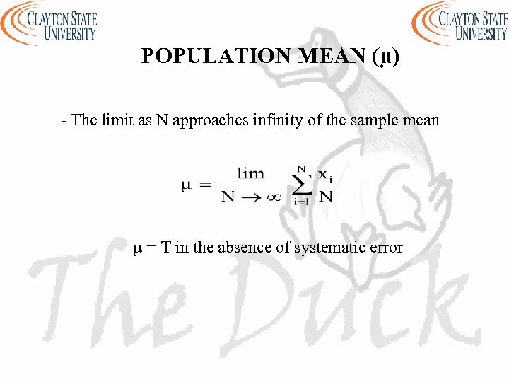POPULATION MEAN (µ) - The limit as N approaches infinity of the sample mean µ = T in the absence of systematic error

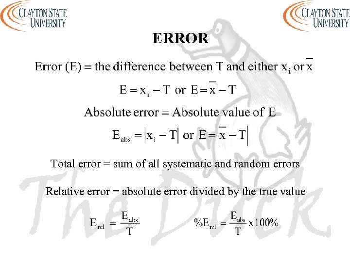ERROR Total error = sum of all systematic and random errors Relative error = absolute error divided by the true value

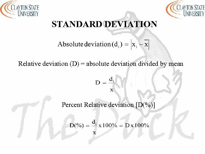STANDARD DEVIATION Relative deviation (D) = absolute deviation divided by mean Percent Relative deviation [D(%)]

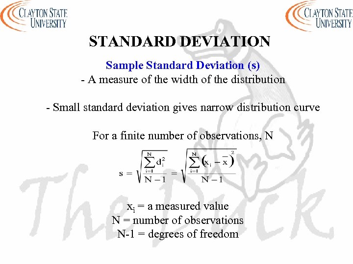STANDARD DEVIATION Sample Standard Deviation (s) - A measure of the width of the distribution - Small standard deviation gives narrow distribution curve For a finite number of observations, N xi = a measured value N = number of observations N-1 = degrees of freedom

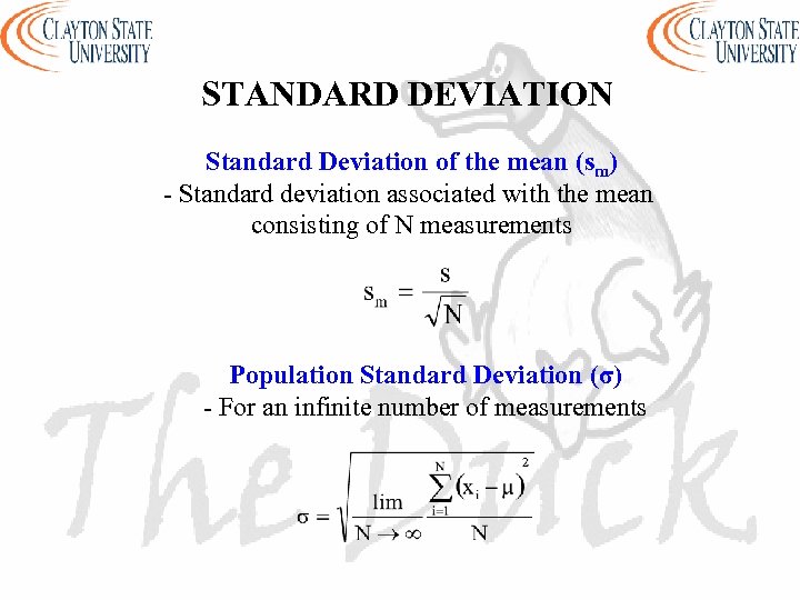STANDARD DEVIATION Standard Deviation of the mean (sm) - Standard deviation associated with the mean consisting of N measurements Population Standard Deviation (σ) - For an infinite number of measurements

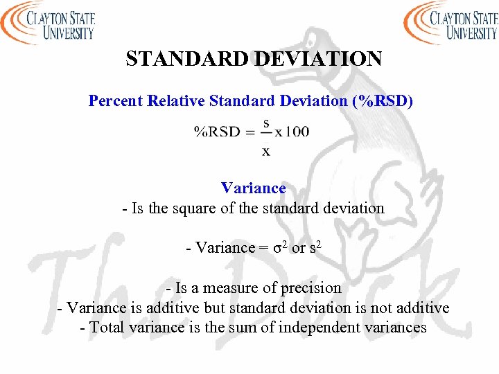STANDARD DEVIATION Percent Relative Standard Deviation (%RSD) Variance - Is the square of the standard deviation - Variance = σ2 or s 2 - Is a measure of precision - Variance is additive but standard deviation is not additive - Total variance is the sum of independent variances

QUANTIFYING RANDOM ERROR Median - The middle number in a series of measurements arranged in increasing order - The average of the two middle numbers if the number of measurements is even Mode - The value that occurs the most frequently Range - The difference between the highest and the lowest values

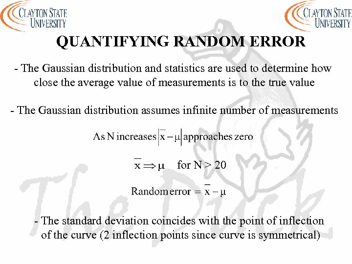QUANTIFYING RANDOM ERROR - The Gaussian distribution and statistics are used to determine how close the average value of measurements is to the true value - The Gaussian distribution assumes infinite number of measurements for N > 20 - The standard deviation coincides with the point of inflection of the curve (2 inflection points since curve is symmetrical)

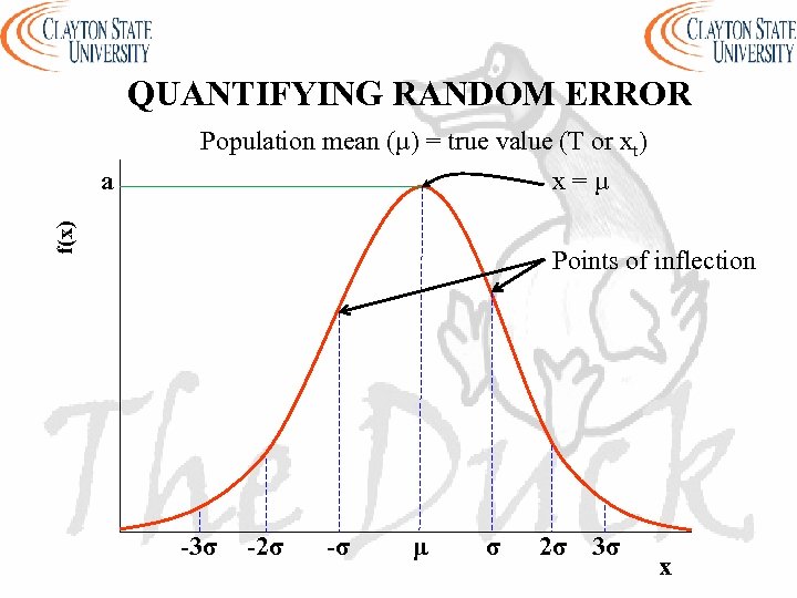QUANTIFYING RANDOM ERROR Population mean (µ) = true value (T or xt) x=µ f(x) a Points of inflection -3σ -2σ -σ μ σ 2σ 3σ x

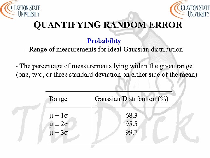QUANTIFYING RANDOM ERROR Probability - Range of measurements for ideal Gaussian distribution - The percentage of measurements lying within the given range (one, two, or three standard deviation on either side of the mean) Range Gaussian Distribution (%) µ ± 1σ µ ± 2σ µ ± 3σ 68. 3 95. 5 99. 7

QUANTIFYING RANDOM ERROR - The average measurement is reported as: mean ± standard deviation - Mean and standard deviation should have the same number of decimal places In the absence of determinate error and if N > 20 - 68. 3% of measurements of xi will fall within x = µ ± σ - (68. 3% of the area under the curve lies in the range of x) - 95. 5% of measurements of xi will fall within x = µ ± 2σ - 99. 7% of measurements of xi will fall within x = µ ± 3σ

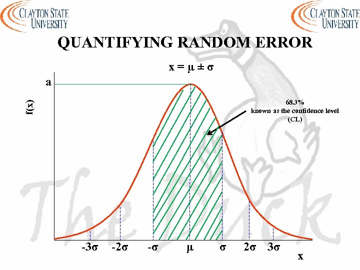QUANTIFYING RANDOM ERROR x=µ±σ a f(x) 68. 3% known as the confidence level (CL) -3σ -2σ -σ μ σ 2σ 3σ x

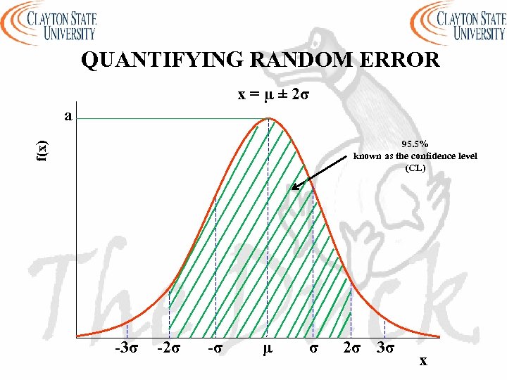QUANTIFYING RANDOM ERROR x = µ ± 2σ a f(x) 95. 5% known as the confidence level (CL) -3σ -2σ -σ μ σ 2σ 3σ x

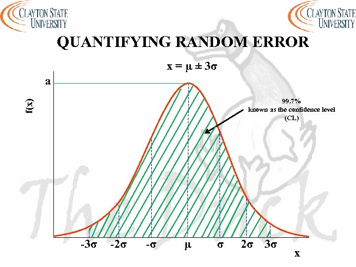QUANTIFYING RANDOM ERROR x = µ ± 3σ a f(x) 99. 7% known as the confidence level (CL) -3σ -2σ -σ μ σ 2σ 3σ x

QUANTIFYING RANDOM ERROR Short-term Precision - Analysis run at the same time by the same analyst using the same instrument and same chemicals Long-term Precision - Compiled results over several months on a regular basis Repeatability - Short-term precision under same operating conditions

QUANTIFYING RANDOM ERROR Reproducibility - Ability of multiple laboratories to obtain same results on a given sample Ruggedness - Degree of reproducibility of results by one laboratory under different conditions (long-term precision) Robustness (Reliability) - Reliable accuracy and precision under small changes in condition

CONFIDENCE LIMITS - Refers to the extremes of the confidence interval (the range) - Range of values within which there is a specified probability of finding the true mean (µ) at a given CL - CL is an indicator of how close the sample mean lies to the population mean µ = x ± zσ

CONFIDENCE LIMITS µ = x ± zσ If z = 1 we are 68. 3% confident that x lies within ±σ of the true value If z = 2 we are 95. 5% confident that x lies within ± 2σ of the true value If z = 3 we are 99. 7% confident that x lies within ± 3σ of the true value

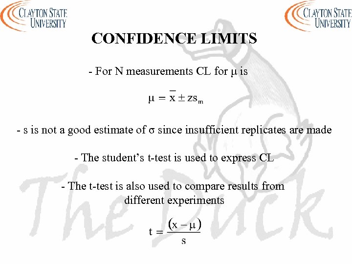CONFIDENCE LIMITS - For N measurements CL for µ is - s is not a good estimate of σ since insufficient replicates are made - The student’s t-test is used to express CL - The t-test is also used to compare results from different experiments

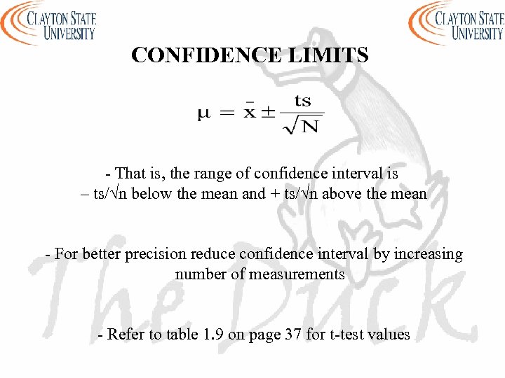CONFIDENCE LIMITS - That is, the range of confidence interval is – ts/√n below the mean and + ts/√n above the mean - For better precision reduce confidence interval by increasing number of measurements - Refer to table 1. 9 on page 37 for t-test values

CONFIDENCE LIMITS To test for comparison of Means - Calculate the pooled standard deviation (spooled) - Calculate t - Compare the calculated t to the value of t from the table - The two results are significantly different if the calculated t is greater than the tabulated t at 95% confidence level (that is tcal > ttab at 95% CL)

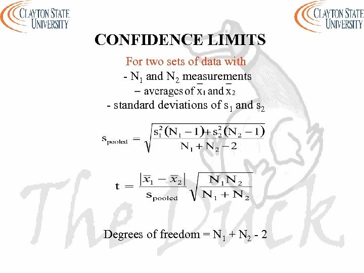CONFIDENCE LIMITS For two sets of data with - N 1 and N 2 measurements - standard deviations of s 1 and s 2 Degrees of freedom = N 1 + N 2 - 2

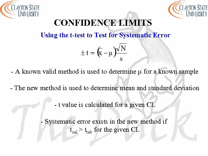CONFIDENCE LIMITS Using the t-test to Test for Systematic Error - A known valid method is used to determine µ for a known sample - The new method is used to determine mean and standard deviation - t value is calculated for a given CL - Systematic error exists in the new method if tcal > ttab for the given CL

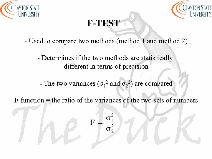F-TEST - Used to compare two methods (method 1 and method 2) - Determines if the two methods are statistically different in terms of precision - The two variances (σ12 and σ22) are compared F-function = the ratio of the variances of the two sets of numbers

F-TEST - Ratio should be greater than 1 (i. e. σ12 > σ22) - F values are found in tables (make use of two degrees of freedom) - Table 1. 10 on page 39 of text book Fcal > Ftab implies there is a significant difference between the two methods Fcal = calculated F value Ftab = tabulated F value

REJECTION OF RESULTS Outlier - A replicate result that is out of the line - A result that is far from other results - Is either the highest value or the lowest value in a set of data - There should be a justification for discarding the outlier - The outlier is rejected if it is > ± 4σ from the mean - The outlier is not included in calculating the mean and standard deviation - A new σ should be calculated that includes outlier if it is < ± 4σ

REJECTION OF RESULTS Q – Test - Used for small data sets - 90% CL is typically used - Arrange data in increasing order - Calculate range = highest value – lowest value - Calculate gap = |suspected value – nearest value| - Calculate Q ratio = gap/range - Reject outlier if Qcal > Qtab - Q tables are available

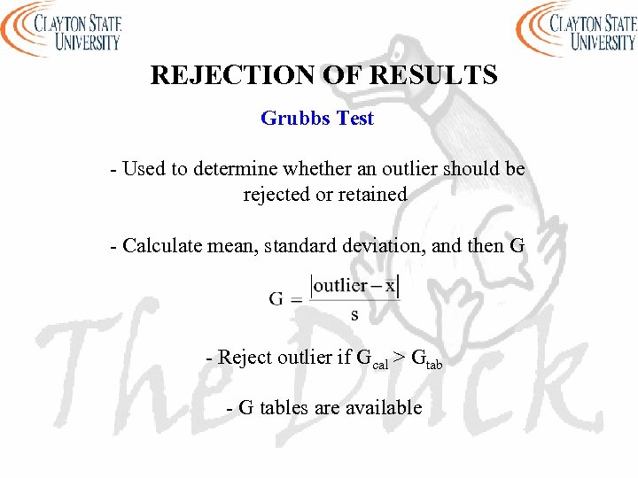REJECTION OF RESULTS Grubbs Test - Used to determine whether an outlier should be rejected or retained - Calculate mean, standard deviation, and then G - Reject outlier if Gcal > Gtab - G tables are available

PERFORMING THE EXPERIMENT Detector - Records the signal (change in the system that is related to the magnitude of the physical parameter being measured) - Can measure physical, chemical or electrical changes Transducer (Sensor) - Detector that converts nonelectrical signals to electrical signals and vice versa

PERFORMING THE EXPERIMENT Signals and Noise - A detector makes measurements and detector response is converted to an electrical signal - The electrical signal is related to the chemical or physical property being measured, which is related to the amount of analyte - There should be no signal when no analyte is present - Signals should be smooth but are practically not smooth due to noise

PERFORMING THE EXPERIMENT Signals and Noise can originate from - Power fluctuations - Radio stations - Electrical motors - Building vibrations - Other instruments nearby

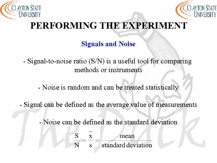PERFORMING THE EXPERIMENT Signals and Noise - Signal-to-noise ratio (S/N) is a useful tool for comparing methods or instruments - Noise is random and can be treated statistically - Signal can be defined as the average value of measurements - Noise can be defined as the standard deviation

PERFORMING THE EXPERIMENT Types of Noise 1. White Noise - Two types Thermal Noise - Due to random motions of charge carriers (electrons) which result in voltage fluctuations Shot Noise - When charge carriers cross a junction in an electrical circuit

PERFORMING THE EXPERIMENT Types of Noise 2. Drift (Flicker) Noise (origin is not well understood) 3. Noise due to surroundings (vibrations) - Signal is enhanced or noise is reduced or both to increase S/N - Hardware and software approaches are available - Another approach is the use of Fourier Transform (FT) or Fast Fourier Transform (FFT) which discriminates signals from noise (FT-IR, FT-NMR, FT-MS)

CALIBRATION CURVES Calibration - The process of establishing the relationship between the measured signals and known concentrations of analyte - Calibration standards: known concentrations of analyte - Calibration standards at different concentrations are prepared and measured - Magnitude of signals are plotted against concentration - Equation relating signal and concentration is obtained and can be used to determine the concentration of unknown analyte after measuring its signal

CALIBRATION CURVES - Many calibration curves have a linear range with the relation equation in the form y = mx + b - The method of least squares or the spreadsheet may be used - m is the slope and b is the vertical (signal) intercept - The slope is usually the sensitivity of the analytical method - R = correlation coefficient (R 2 is between 0 and 1) - Perfect fit of data (direct relation) if R 2 is closer to 1

BEST STRAIGHT LINE (METHOD OF LEAST SQUARES) The equation of a straight line y = mx + b m is the slope ( y/ x) b is the y-intercept (where the line crosses the y-axis)

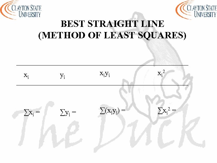
BEST STRAIGHT LINE (METHOD OF LEAST SQUARES) The method of least squares - finds the best straight line - adjusts the line to minimize the vertical deviations Only vertical deviations are adjusted because - experimental uncertainties in y values > in x values - calculations for minimizing vertical deviations are easier

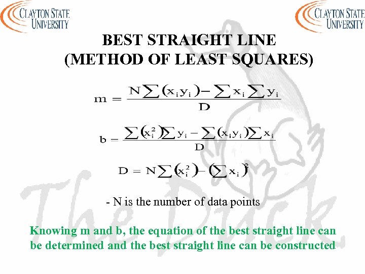BEST STRAIGHT LINE (METHOD OF LEAST SQUARES) - N is the number of data points Knowing m and b, the equation of the best straight line can be determined and the best straight line can be constructed

BEST STRAIGHT LINE (METHOD OF LEAST SQUARES) xi yi xi 2 ∑xi = ∑yi = ∑(xiyi) = ∑xi 2 =

ASSESSING THE DATA A good analytical method should be - both accurate and precise - reliable and robust - It is not a good practice to extrapolate above the highest standard or below the lowest standard - These regions may not be in the linear range - Dilute higher concentrations and concentrate lower concentrations of analyte to bring them into the working range

ASSESSING THE DATA Limit of Detection (LOD) - The lowest concentration of an analyte that can be detected - Increasing concentration of analyte decreases signal due to noise - Signal can no longer be distinguished from noise at a point - LOD does not necessarily mean concentration can be measured and quantified

ASSESSING THE DATA Limit of Detection (LOD) - Can be considered to be the concentration of analyte that gives a signal that is equal to 2 or 3 times the standard deviation of the blank - Concentration at which S/N = 2 at 95% CL or S/N = 3 at 99% CL - 3σ is more common and used by regulatory methods (e. g. EPA)

ASSESSING THE DATA Limit of Quantification (LOQ) - The lowest concentration of an analyte in a sample that can be determined quantitatively with a given accuracy and precision - Precision is poor at or near LOD - LOQ is higher than LOD and has better precision - LOQ is the concentration equivalent to S/N = 10/1 - LOQ is also defined as 10 x σblank