Information Retrieval and Map -Reduce Implementations Adopted from

Information Retrieval and Map -Reduce Implementations Adopted from Jimmy Lin’s slides, which is licensed under a Creative Commons Attribution-Noncommercial-Share Alike 3. 0 United States

Roadmap ¢ Introduction to information retrieval ¢ Basics of indexing and retrieval ¢ Inverted indexing in Map. Reduce ¢ Retrieval at scale

First, nomenclature… ¢ Information retrieval (IR) l l ¢ What do we search? l l ¢ Focus on textual information (= text/document retrieval) Other possibilities include image, video, music, … Generically, “collections” Less-frequently used, “corpora” What do we find? l l Generically, “documents” Even though we may be referring to web pages, PDFs, Power. Point slides, paragraphs, etc.

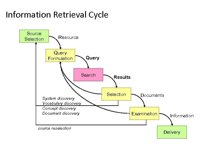Information Retrieval Cycle Source Selection Resource Query Formulation Query Search System discovery Vocabulary discovery Concept discovery Document discovery source reselection Results Selection Documents Examination Information Delivery

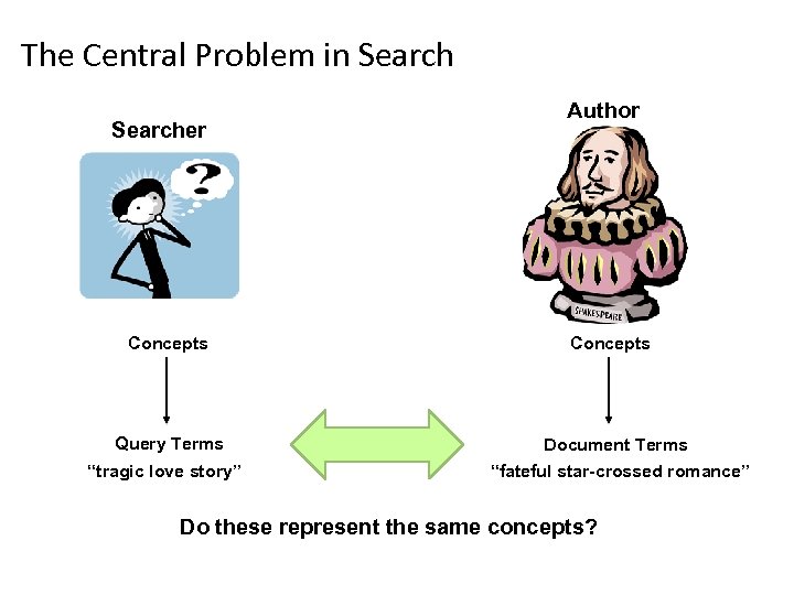The Central Problem in Searcher Concepts Query Terms “tragic love story” Author Concepts Document Terms “fateful star-crossed romance” Do these represent the same concepts?

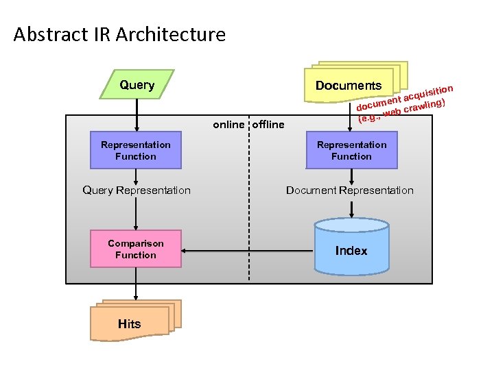Abstract IR Architecture Query Documents online offline sition acqui ) ent g docum eb crawlin w (e. g. , Representation Function Query Representation Document Representation Comparison Function Index Hits

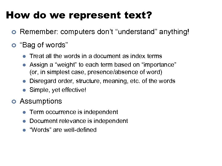How do we represent text? ¢ Remember: computers don’t “understand” anything! ¢ “Bag of words” l l ¢ Treat all the words in a document as index terms Assign a “weight” to each term based on “importance” (or, in simplest case, presence/absence of word) Disregard order, structure, meaning, etc. of the words Simple, yet effective! Assumptions l l l Term occurrence is independent Document relevance is independent “Words” are well-defined

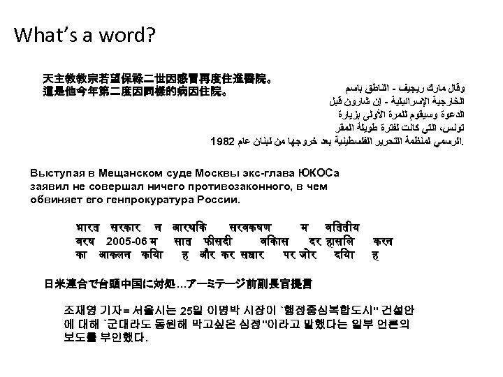What’s a word? 天主教教宗若望保祿二世因感冒再度住進醫院。 這是他今年第二度因同樣的病因住院。 ﻭﻗﺎﻝ ﻣﺎﺭﻙ ﺭﻳﺠﻴﻒ - ﺍﻟﻨﺎﻃﻖ ﺑﺎﺳﻢ ﺍﻟﺨﺎﺭﺟﻴﺔ ﺍﻹﺳﺮﺍﺋﻴﻠﻴﺔ - ﺇﻥ ﺷﺎﺭﻭﻥ ﻗﺒﻞ ﺍﻟﺪﻋﻮﺓ ﻭﺳﻴﻘﻮﻡ ﻟﻠﻤﺮﺓ ﺍﻷﻮﻟﻰ ﺑﺰﻳﺎﺭﺓ ﺗﻮﻧﺲ، ﺍﻟﺘﻲ ﻛﺎﻧﺖ ﻟﻔﺘﺮﺓ ﻃﻮﻳﻠﺔ ﺍﻟﻤﻘﺮ 1982 . ﺍﻟﺮﺳﻤﻲ ﻟﻤﻨﻈﻤﺔ ﺍﻟﺘﺤﺮﻳﺮ ﺍﻟﻔﻠﺴﻄﻴﻨﻴﺔ ﺑﻌﺪ ﺧﺮﻭﺟﻬﺎ ﻣﻦ ﻟﺒﻨﺎﻥ ﻋﺎﻡ Выступая в Мещанском суде Москвы экс-глава ЮКОСа заявил не совершал ничего противозаконного, в чем обвиняет его генпрокуратура России. भ रत सरक र न आरथ क सरवकषण म व तत य वरष 2005 -06 म स त फ सद व क स दर ह स ल क आकलन क य ह और कर सध र पर ज र द य करन ह 日米連合で台頭中国に対処…アーミテージ前副長官提言 조재영 기자= 서울시는 25일 이명박 시장이 `행정중심복합도시'' 건설안 에 대해 `군대라도 동원해 막고싶은 심정''이라고 말했다는 일부 언론의 보도를 부인했다.

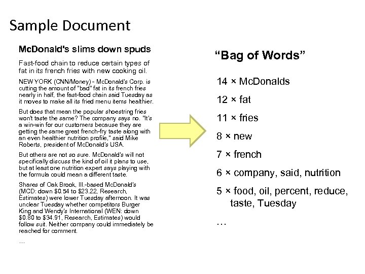Sample Document Mc. Donald's slims down spuds Fast-food chain to reduce certain types of fat in its french fries with new cooking oil. NEW YORK (CNN/Money) - Mc. Donald's Corp. is cutting the amount of "bad" fat in its french fries nearly in half, the fast-food chain said Tuesday as it moves to make all its fried menu items healthier. But does that mean the popular shoestring fries won't taste the same? The company says no. "It's a win-win for our customers because they are getting the same great french-fry taste along with an even healthier nutrition profile, " said Mike Roberts, president of Mc. Donald's USA. But others are not so sure. Mc. Donald's will not specifically discuss the kind of oil it plans to use, but at least one nutrition expert says playing with the formula could mean a different taste. Shares of Oak Brook, Ill. -based Mc. Donald's (MCD: down $0. 54 to $23. 22, Research, Estimates) were lower Tuesday afternoon. It was unclear Tuesday whether competitors Burger King and Wendy's International (WEN: down $0. 80 to $34. 91, Research, Estimates) would follow suit. Neither company could immediately be reached for comment. … “Bag of Words” 14 × Mc. Donalds 12 × fat 11 × fries 8 × new 7 × french 6 × company, said, nutrition 5 × food, oil, percent, reduce, taste, Tuesday …

Information retrieval models ¢ An IR model governs how a document and a query are represented and how the relevance of a document to a user query is defined. ¢ Main models: l l Boolean model Vector space model Statistical language model etc 10

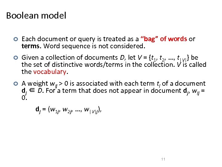Boolean model ¢ Each document or query is treated as a “bag” of words or terms. Word sequence is not considered. ¢ Given a collection of documents D, let V = {t 1, t 2, . . . , t|V|} be the set of distinctive words/terms in the collection. V is called the vocabulary. ¢ A weight wij > 0 is associated with each term ti of a document dj ∈ D. For a term that does not appear in document dj, wij = 0. dj = (w 1 j, w 2 j, . . . , w|V|j), 11

Boolean model (contd) ¢ Query terms are combined logically using the Boolean operators AND, OR, and NOT. l ¢ Retrieval l l ¢ E. g. , ((data AND mining) AND (NOT text)) Given a Boolean query, the system retrieves every document that makes the query logically true. Called exact match. The retrieval results are usually quite poor because term frequency is not considered. 12

Sec. 1. 3 Boolean queries: Exact match • The Boolean retrieval model is being able to ask a query that is a Boolean expression: – Boolean Queries are queries using AND, OR and NOT to join query terms • Views each document as a set of words • Is precise: document matches condition or not. – • • Perhaps the simplest model to build an IR system on Primary commercial retrieval tool for 3 decades. Many search systems you still use are Boolean: – Email, library catalog, Mac OS X Spotlight 13

Strengths and Weaknesses ¢ Strengths l l l ¢ Precise, if you know the right strategies Precise, if you have an idea of what you’re looking for Implementations are fast and efficient Weaknesses l l l Users must learn Boolean logic insufficient to capture the richness of language No control over size of result set: either too many hits or none When do you stop reading? All documents in the result set are considered “equally good” What about partial matches? Documents that “don’t quite match” the query may be useful also

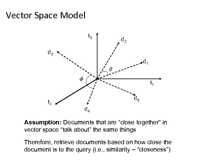Vector Space Model t 3 d 2 d 3 d 1 θ φ t 1 d 5 t 2 d 4 Assumption: Documents that are “close together” in vector space “talk about” the same things Therefore, retrieve documents based on how close the document is to the query (i. e. , similarity ~ “closeness”)

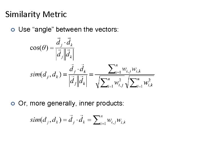Similarity Metric ¢ Use “angle” between the vectors: ¢ Or, more generally, inner products:

Vector space model ¢ Documents are also treated as a “bag” of words or terms. ¢ Each document is represented as a vector. ¢ However, the term weights are no longer 0 or 1. Each term weight is computed based on some variations of TF or TF-IDF scheme. 17

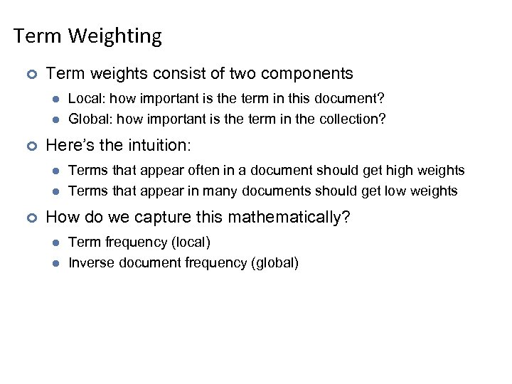Term Weighting ¢ Term weights consist of two components l l ¢ Here’s the intuition: l l ¢ Local: how important is the term in this document? Global: how important is the term in the collection? Terms that appear often in a document should get high weights Terms that appear in many documents should get low weights How do we capture this mathematically? l l Term frequency (local) Inverse document frequency (global)

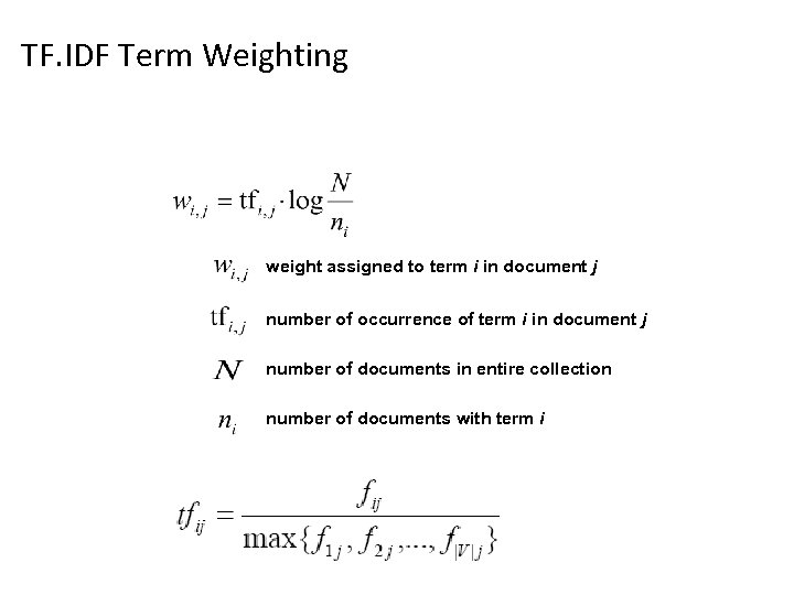TF. IDF Term Weighting weight assigned to term i in document j number of occurrence of term i in document j number of documents in entire collection number of documents with term i

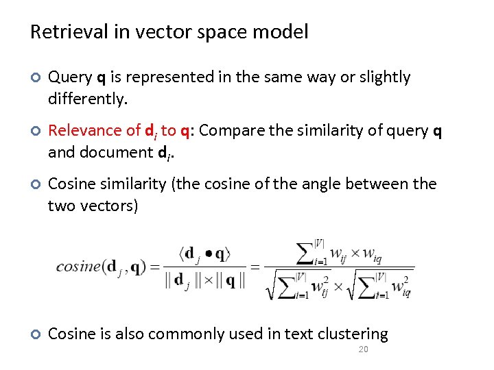Retrieval in vector space model ¢ Query q is represented in the same way or slightly differently. ¢ Relevance of di to q: Compare the similarity of query q and document di. ¢ Cosine similarity (the cosine of the angle between the two vectors) ¢ Cosine is also commonly used in text clustering 20

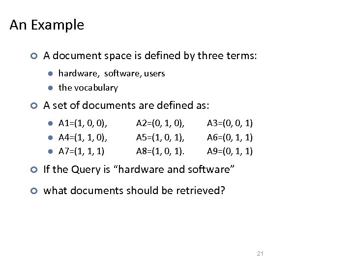An Example ¢ A document space is defined by three terms: l l ¢ hardware, software, users the vocabulary A set of documents are defined as: l l l A 1=(1, 0, 0), A 4=(1, 1, 0), A 7=(1, 1, 1) A 2=(0, 1, 0), A 5=(1, 0, 1), A 8=(1, 0, 1). A 3=(0, 0, 1) A 6=(0, 1, 1) A 9=(0, 1, 1) ¢ If the Query is “hardware and software” ¢ what documents should be retrieved? 21

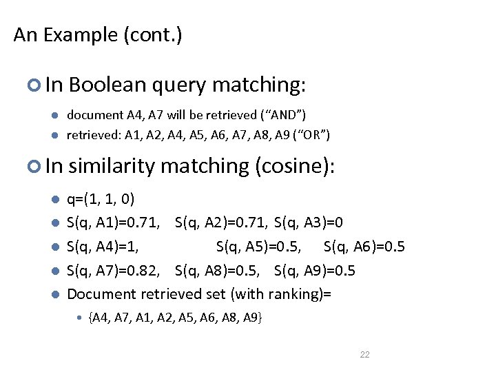An Example (cont. ) ¢ In Boolean query matching: l l document A 4, A 7 will be retrieved (“AND”) retrieved: A 1, A 2, A 4, A 5, A 6, A 7, A 8, A 9 (“OR”) ¢ In similarity matching (cosine): l l l q=(1, 1, 0) S(q, A 1)=0. 71, S(q, A 2)=0. 71, S(q, A 3)=0 S(q, A 4)=1, S(q, A 5)=0. 5, S(q, A 6)=0. 5 S(q, A 7)=0. 82, S(q, A 8)=0. 5, S(q, A 9)=0. 5 Document retrieved set (with ranking)= • {A 4, A 7, A 1, A 2, A 5, A 6, A 8, A 9} 22

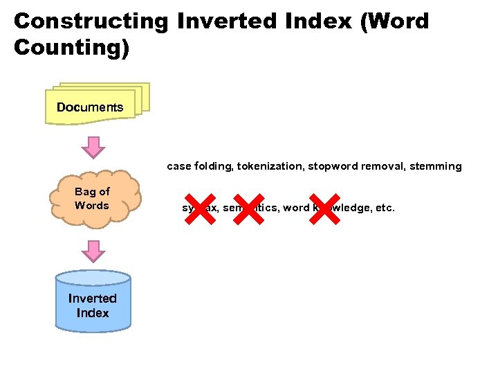Constructing Inverted Index (Word Counting) Documents case folding, tokenization, stopword removal, stemming Bag of Words Inverted Index syntax, semantics, word knowledge, etc.

Stopwords removal • Many of the most frequently used words in English are useless in IR and text mining – these words are called stop words. – the, of, and, to, …. – Typically about 400 to 500 such words – For an application, an additional domain specific stopwords list may be constructed • Why do we need to remove stopwords? – Reduce indexing (or data) file size • stopwords accounts 20 -30% of total word counts. – Improve efficiency and effectiveness • stopwords are not useful for searching or text mining • they may also confuse the retrieval system. 24

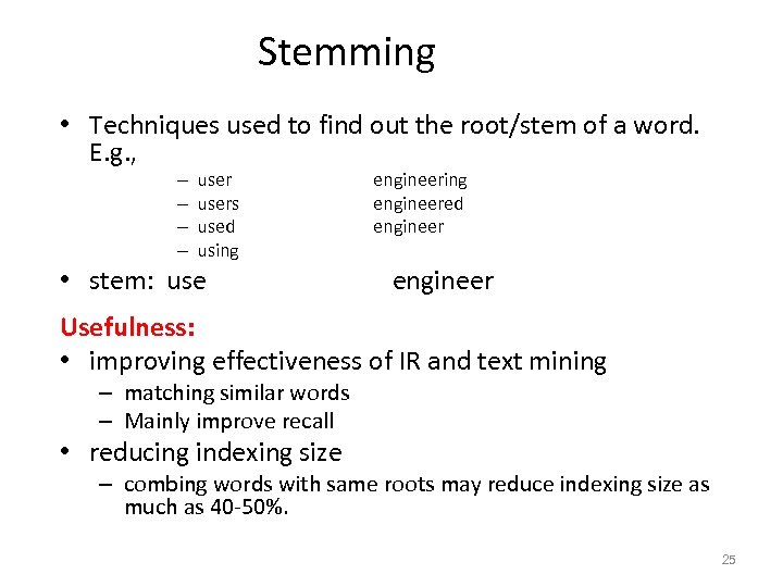Stemming • Techniques used to find out the root/stem of a word. E. g. , – – users used using • stem: use engineering engineered engineer Usefulness: • improving effectiveness of IR and text mining – matching similar words – Mainly improve recall • reducing indexing size – combing words with same roots may reduce indexing size as much as 40 -50%. 25

Basic stemming methods Using a set of rules. E. g. , • remove ending – if a word ends with a consonant other than s, followed by an s, then delete s. – if a word ends in es, drop the s. – if a word ends in ing, delete the ing unless the remaining word consists only of one letter or of th. – If a word ends with ed, preceded by a consonant, delete the ed unless this leaves only a single letter. – …. . . • transform words – if a word ends with “ies” but not “eies” or “aies” then “ies --> y. ” 26

Inverted index ¢ The inverted index of a document collection is basically a data structure that l ¢ attaches each distinctive term with a list of all documents that contains the term. Thus, in retrieval, it takes constant time to l l find the documents that contains a query term. multiple query terms are also easy handle as we will see soon. 27

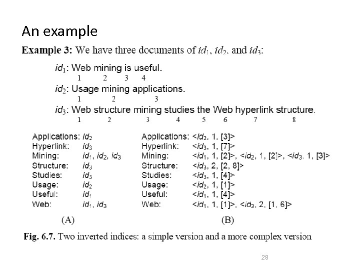An example 28

Search using inverted index Given a query q, search has the following steps: • Step 1 (vocabulary search): find each term/word in q in the inverted index. • Step 2 (results merging): Merge results to find documents that contain all or some of the words/terms in q. • Step 3 (Rank score computation): To rank the resulting documents/pages, using, – – content-based ranking link-based ranking 29

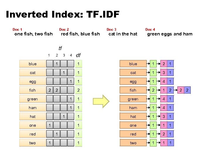
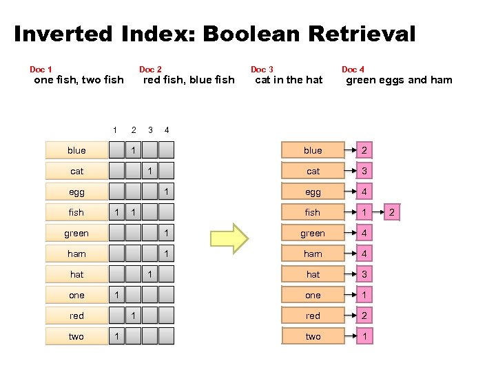Inverted Index: Boolean Retrieval Doc 1 Doc 2 one fish, two fish 1 blue red fish, blue fish 2 3 1 3 egg 4 fish 1 2 cat 1 1 green eggs and ham blue egg fish cat in the hat Doc 4 4 1 cat Doc 3 1 green 4 ham 1 ham 4 hat 3 one 1 red 2 two 1 hat one 1 1 red two 1 1 2

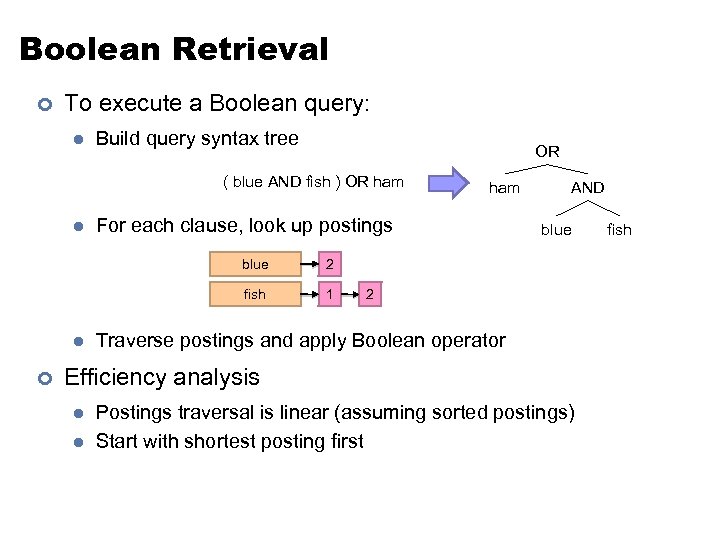Boolean Retrieval ¢ To execute a Boolean query: l Build query syntax tree OR ( blue AND fish ) OR ham l For each clause, look up postings blue ¢ 1 AND blue 2 fish l ham 2 Traverse postings and apply Boolean operator Efficiency analysis l l Postings traversal is linear (assuming sorted postings) Start with shortest posting first fish

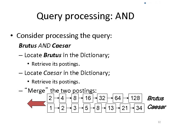n. Sec. 1. 3 Query processing: AND • Consider processing the query: Brutus AND Caesar – Locate Brutus in the Dictionary; • Retrieve its postings. – Locate Caesar in the Dictionary; • Retrieve its postings. – “Merge” the two postings: 2 4 8 16 1 2 3 5 32 8 64 13 Brutus 34 Caesar 128 21 32

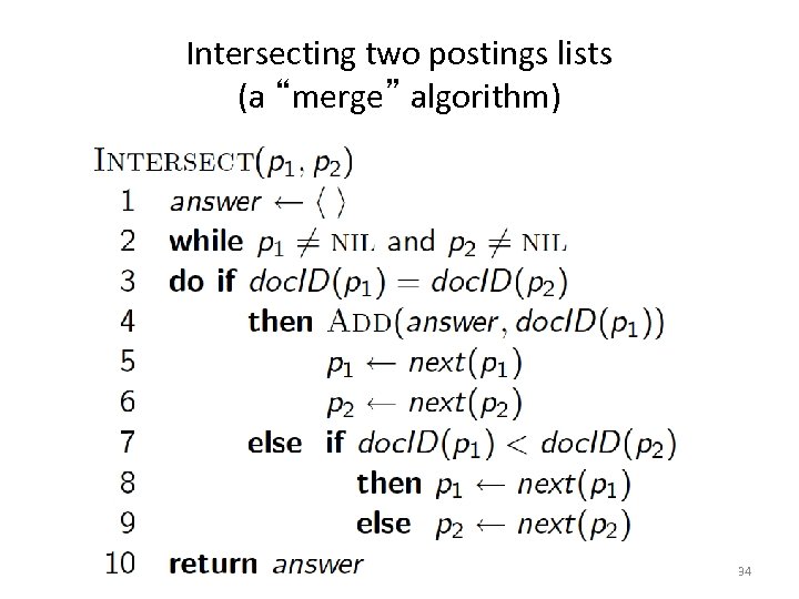
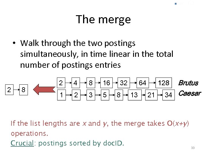n. Sec. 1. 3 The merge • Walk through the two postings simultaneously, in time linear in the total number of postings entries 2 8 2 4 8 16 1 2 3 5 32 8 13 Brutus 34 Caesar 128 64 21 If the list lengths are x and y, the merge takes O(x+y) operations. Crucial: postings sorted by doc. ID. 33

Intersecting two postings lists (a “merge” algorithm) 34

Inverted Index: TF. IDF Doc 1 Doc 2 one fish, two fish red fish, blue fish Doc 3 cat in the hat Doc 4 green eggs and ham tf 1 blue 2 3 1 2 1 cat 1 3 1 1 egg 1 4 1 2 egg blue 1 1 2 df 1 1 cat fish 4 fish 2 1 2 green 1 1 green 1 4 1 ham 1 4 1 1 hat 1 3 1 1 one 1 1 red 1 2 1 1 two 1 1 1 hat one 1 1 red two 1 1 2 2

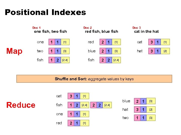
Positional Indexes ¢ Store term position in postings ¢ Supports richer queries (e. g. , proximity) ¢ Naturally, leads to larger indexes…

Inverted Index: Positional Information Doc 1 Doc 2 one fish, two fish red fish, blue fish Doc 3 cat in the hat Doc 4 green eggs and ham tf 1 blue 2 3 1 2 1 [3] cat 1 3 1 [1] 1 egg 1 4 1 [2] 2 egg blue 1 1 2 df 1 1 cat fish 4 fish 2 1 2 [2, 4] green 1 1 green 1 4 1 [1] ham 1 1 ham 1 4 1 [3] 1 hat 1 3 1 [2] 1 one 1 1 1 [1] 1 red 1 2 1 [1] 1 two 1 1 1 [3] hat one 1 1 red two 1 1 2 2 [2, 4]

Retrieval in a Nutshell ¢ Look up postings lists corresponding to query terms ¢ Traverse postings for each query term ¢ Store partial query-document scores in accumulators ¢ Select top k results to return

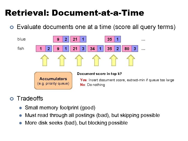Retrieval: Document-at-a-Time ¢ Evaluate documents one at a time (score all query terms) blue fish 9 1 2 2 21 1 9 1 21 3 35 34 1 35 2 … 1 80 3 … Document score in top k? Accumulators (e. g. priority queue) ¢ Yes: Insert document score, extract-min if queue too large No: Do nothing Tradeoffs l l l Small memory footprint (good) Must read through all postings (bad), but skipping possible More disk seeks (bad), but blocking possible

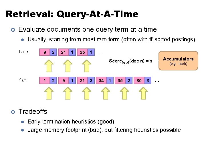Retrieval: Query-At-A-Time ¢ Evaluate documents one query term at a time l Usually, starting from most rare term (often with tf-sorted postings) blue 9 2 21 1 35 1 … Accumulators Score{q=x}(doc n) = s fish ¢ 1 2 9 1 21 3 34 1 35 2 80 3 (e. g. , hash) … Tradeoffs l l Early termination heuristics (good) Large memory footprint (bad), but filtering heuristics possible

Map. Reduce it? ¢ The indexing problem l l l ¢ P erfect for M Scalability is critical ap. Reduce! Must be relatively fast, but need not be real time Fundamentally a batch operation Incremental updates may or may not be important For the web, crawling is a challenge in itself The retrieval problem l l Must have sub-second response time For the web, only need relatively few results ot so good… Uh… n

Indexing: Performance Analysis ¢ Fundamentally, a large sorting problem l l Terms usually fit in memory Postings usually don’t ¢ How is it done on a single machine? ¢ How can it be done with Map. Reduce? ¢ First, let’s characterize the problem size: l l Size of vocabulary Size of postings

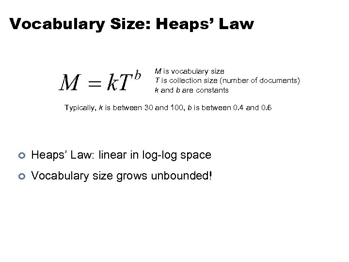Vocabulary Size: Heaps’ Law M is vocabulary size T is collection size (number of documents) k and b are constants Typically, k is between 30 and 100, b is between 0. 4 and 0. 6 ¢ Heaps’ Law: linear in log-log space ¢ Vocabulary size grows unbounded!

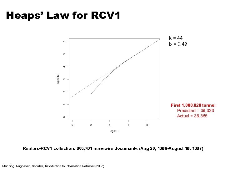Heaps’ Law for RCV 1 k = 44 b = 0. 49 First 1, 000, 020 terms: Predicted = 38, 323 Actual = 38, 365 Reuters-RCV 1 collection: 806, 791 newswire documents (Aug 20, 1996 -August 19, 1997) Manning, Raghavan, Schütze, Introduction to Information Retrieval (2008)

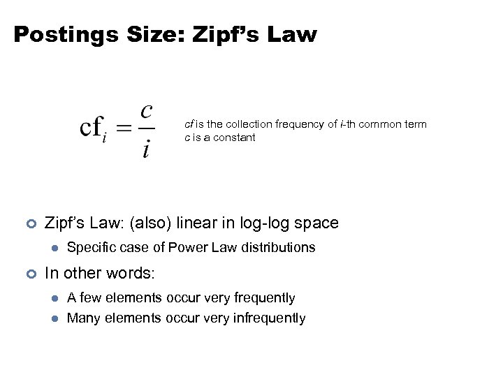Postings Size: Zipf’s Law cf is the collection frequency of i-th common term c is a constant ¢ Zipf’s Law: (also) linear in log-log space l ¢ Specific case of Power Law distributions In other words: l l A few elements occur very frequently Many elements occur very infrequently

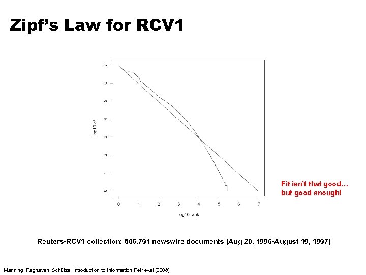Zipf’s Law for RCV 1 Fit isn’t that good… but good enough! Reuters-RCV 1 collection: 806, 791 newswire documents (Aug 20, 1996 -August 19, 1997) Manning, Raghavan, Schütze, Introduction to Information Retrieval (2008)

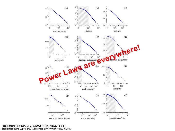ryw ve Law er Pow Figure from: Newman, M. E. J. (2005) “Power laws, Pareto distributions and Zipf's law. ” Contemporary Physics 46: 323– 351. re e sa re! he

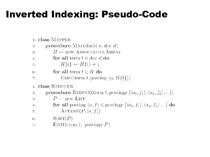
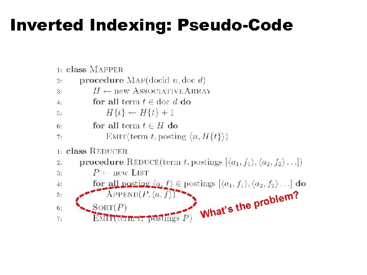
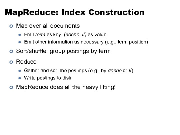Map. Reduce: Index Construction ¢ Map over all documents l l Emit term as key, (docno, tf) as value Emit other information as necessary (e. g. , term position) ¢ Sort/shuffle: group postings by term ¢ Reduce l l ¢ Gather and sort the postings (e. g. , by docno or tf) Write postings to disk Map. Reduce does all the heavy lifting!

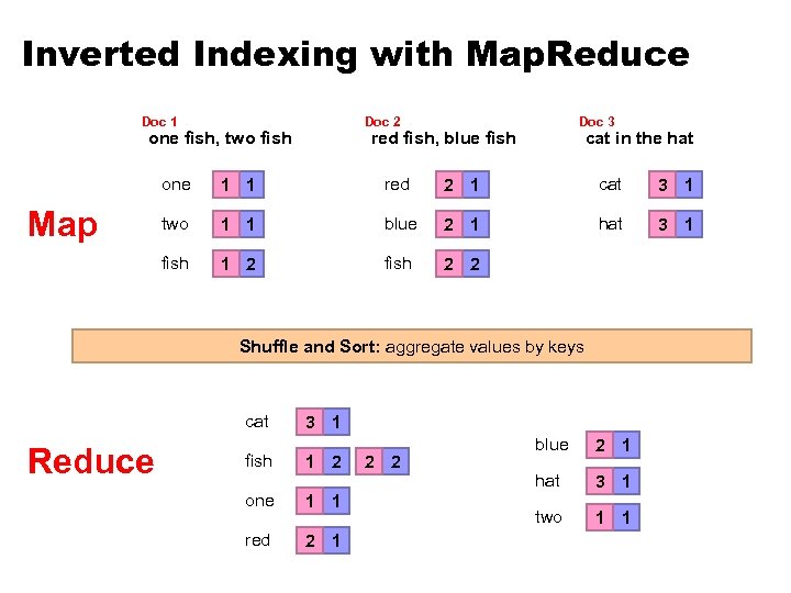Inverted Indexing with Map. Reduce Doc 1 Doc 2 one fish, two fish Doc 3 red fish, blue fish cat in the hat one red 2 1 cat 3 1 two 1 1 blue 2 1 hat 3 1 fish Map 1 1 1 2 fish 2 2 Shuffle and Sort: aggregate values by keys cat Reduce fish 3 1 1 2 one 1 1 red 2 1 2 2 blue 2 1 hat 3 1 two 1 1

Inverted Indexing: Pseudo-Code

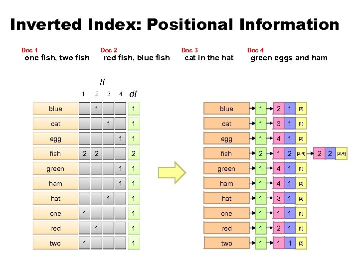
Positional Indexes Doc 1 Doc 2 one fish, two fish Doc 3 red fish, blue fish cat in the hat one [1] red 2 1 [1] cat 3 1 [1] two 1 1 [3] blue 2 1 [3] hat 3 1 [2] fish Map 1 1 1 2 [2, 4] fish 2 2 [2, 4] Shuffle and Sort: aggregate values by keys cat Reduce fish one red 3 1 1 2 1 [1] [2, 4] [1] 2 2 blue 2 1 [3] hat 3 1 [2] two 1 1 [3] [2, 4]

Inverted Indexing: Pseudo-Code ’s What th ? oblem e pr

Scalability Bottleneck ¢ Initial implementation: terms as keys, postings as values l l ¢ Reducers must buffer all postings associated with key (to sort) What if we run out of memory to buffer postings? Uh oh!

Another Try… (key) fish (values) (keys) (values) 1 2 [2, 4] fish 1 [2, 4] 34 1 [23] fish 9 [9] 21 3 [1, 8, 22] fish 21 [1, 8, 22] 35 2 [8, 41] fish 34 [23] 80 3 [2, 9, 76] fish 35 [8, 41] 9 1 [9] fish 80 [2, 9, 76] How is this different? • Let the framework do the sorting • Term frequency implicitly stored • Directly write postings to disk! Where have we seen this before?

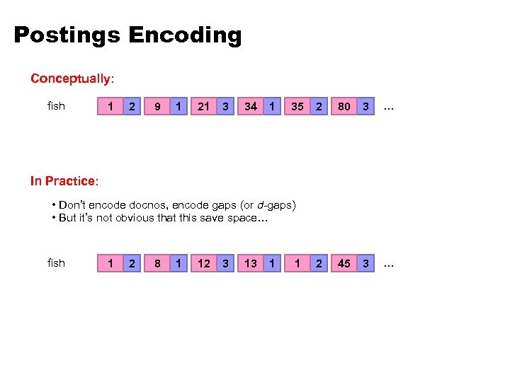Postings Encoding Conceptually: fish 1 2 9 1 21 3 34 1 35 2 80 3 … 2 45 3 … In Practice: • Don’t encode docnos, encode gaps (or d-gaps) • But it’s not obvious that this save space… fish 1 2 8 1 12 3 13 1 1

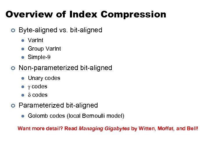Overview of Index Compression ¢ Byte-aligned vs. bit-aligned l l l ¢ Non-parameterized bit-aligned l l l ¢ Var. Int Group Var. Int Simple-9 Unary codes Parameterized bit-aligned l Golomb codes (local Bernoulli model) Want more detail? Read Managing Gigabytes by Witten, Moffat, and Bell!

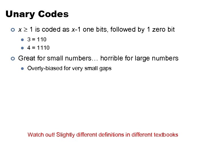Unary Codes ¢ x 1 is coded as x-1 one bits, followed by 1 zero bit l l ¢ 3 = 110 4 = 1110 Great for small numbers… horrible for large numbers l Overly-biased for very small gaps Watch out! Slightly different definitions in different textbooks

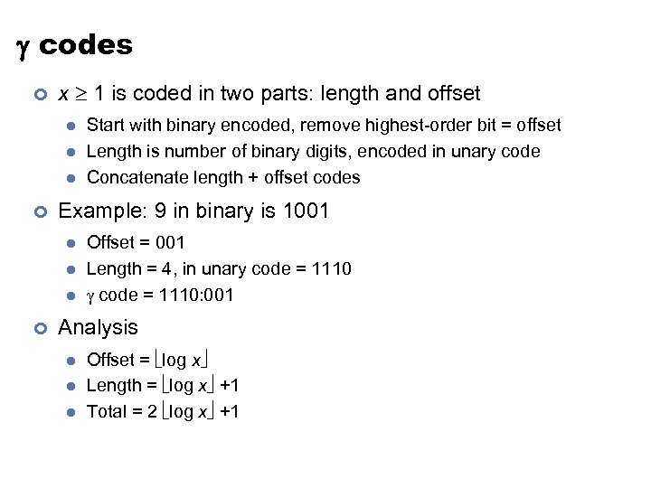codes ¢ x 1 is coded in two parts: length and offset l l l ¢ Example: 9 in binary is 1001 l l l ¢ Start with binary encoded, remove highest-order bit = offset Length is number of binary digits, encoded in unary code Concatenate length + offset codes Offset = 001 Length = 4, in unary code = 1110: 001 Analysis l l l Offset = log x Length = log x +1 Total = 2 log x +1

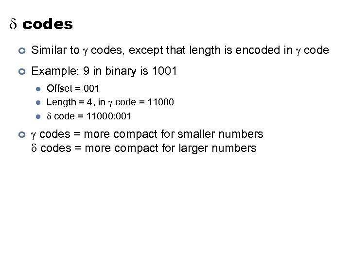codes ¢ Similar to codes, except that length is encoded in code ¢ Example: 9 in binary is 1001 l l l ¢ Offset = 001 Length = 4, in code = 11000: 001 codes = more compact for smaller numbers codes = more compact for larger numbers

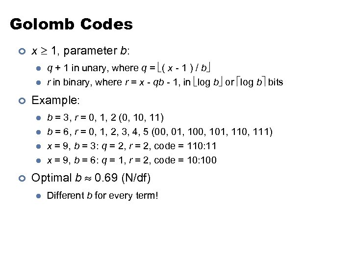Golomb Codes ¢ x 1, parameter b: l l ¢ Example: l l ¢ q + 1 in unary, where q = ( x - 1 ) / b r in binary, where r = x - qb - 1, in log b or log b bits b = 3, r = 0, 1, 2 (0, 11) b = 6, r = 0, 1, 2, 3, 4, 5 (00, 01, 100, 101, 110, 111) x = 9, b = 3: q = 2, r = 2, code = 110: 11 x = 9, b = 6: q = 1, r = 2, code = 10: 100 Optimal b 0. 69 (N/df) l Different b for every term!

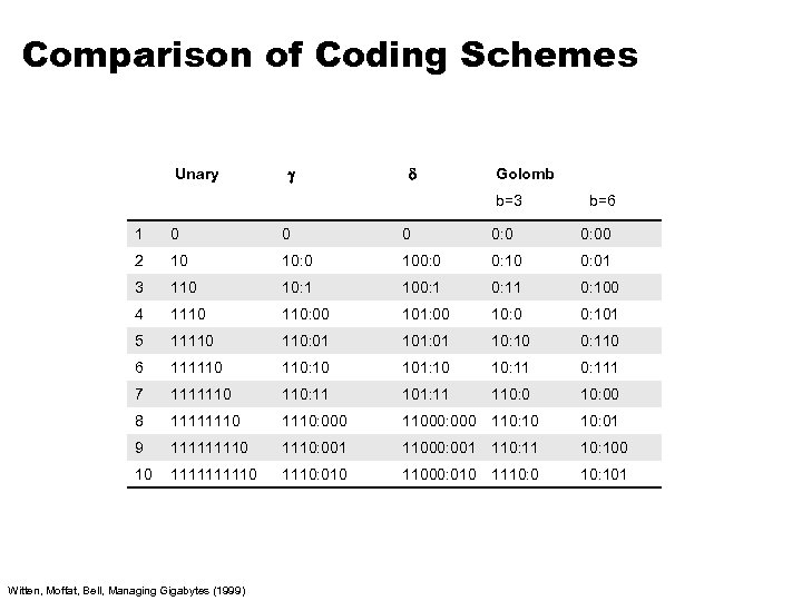Comparison of Coding Schemes Unary Golomb b=3 b=6 1 0 0: 00 2 10 10: 0 100: 0 0: 10 0: 01 3 110 10: 1 100: 100 4 1110 110: 00 101: 00 10: 0 0: 101 5 11110 110: 01 101: 01 10: 10 0: 110 6 111110 110: 10 101: 10 10: 111 7 1111110 110: 11 101: 11 110: 00 8 11111110: 000 11000: 000 110: 10 10: 01 9 11110: 001 11000: 001 110: 11 10: 100 10 111110: 010 11000: 010 1110: 0 10: 101 Witten, Moffat, Bell, Managing Gigabytes (1999)

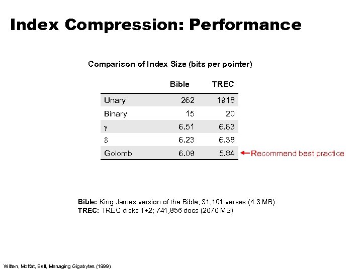Index Compression: Performance Comparison of Index Size (bits per pointer) Bible TREC Unary 262 1918 Binary 15 20 6. 51 6. 63 6. 23 6. 38 Golomb 6. 09 5. 84 Recommend best practice Bible: King James version of the Bible; 31, 101 verses (4. 3 MB) TREC: TREC disks 1+2; 741, 856 docs (2070 MB) Witten, Moffat, Bell, Managing Gigabytes (1999)

Reachability Query and Transitive Closure Representation The problem: Given two vertices u and v in a directed graph G, is there a path from u to v ? 15 14 11 13 10 6 7 3 12 4 1 8 9 ? Query(1, 11) Yes ? Query(3, 9) No 5 2 Directed Graph DAG (directed acyclic graph) by coalescing the strongly connected components

Chicken and Egg? (key) (value) fish 1 [2, 4] fish 9 [9] fish 21 [1, 8, 22] fish 34 [23] We need the df to set b… fish 35 [8, 41] fish 80 [2, 9, 76] But we don’t know the df until we’ve seen all postings! But wait! How do we set the Golomb parameter b? Recall: optimal b 0. 69 (N/df) … Write directly to disk Sound familiar?

Getting the df ¢ In the mapper: l ¢ In the reducer: l ¢ Emit “special” key-value pairs to keep track of df Make sure “special” key-value pairs come first: process them to determine df Remember: proper partitioning!

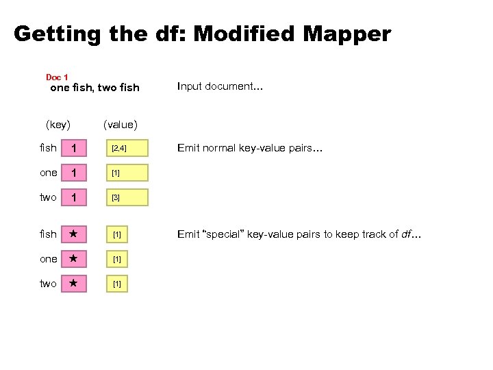Getting the df: Modified Mapper Doc 1 one fish, two fish (key) Input document… (value) fish 1 [2, 4] one 1 [1] two 1 [3] fish [1] one [1] two [1] Emit normal key-value pairs… Emit “special” key-value pairs to keep track of df…

Getting the df: Modified Reducer (key) fish (value) [63] [82] [27] … First, compute the df by summing contributions from all “special” key-value pair… Compute Golomb parameter b… fish 1 [2, 4] fish 9 [9] fish 21 [1, 8, 22] fish 34 [23] fish 35 [8, 41] fish 80 [2, 9, 76] … Important: properly define sort order to make sure “special” key-value pairs come first! Write postings directly to disk Where have we seen this before?

Map. Reduce it? ¢ The indexing problem l l l ¢ Scalability is paramount Must be relatively fast, but need not be real time Fundamentally a batch operation Incremental updates may or may not be important For the web, crawling is a challenge in itself The retrieval problem l l Just covered Must have sub-second response time For the web, only need relatively few results Now

Retrieval with Map. Reduce? ¢ Map. Reduce is fundamentally batch-oriented l l ¢ Optimized for throughput, not latency Startup of mappers and reducers is expensive Map. Reduce is not suitable for real-time queries! l Use separate infrastructure for retrieval…

Important Ideas ¢ Partitioning (for scalability) ¢ Replication (for redundancy) ¢ Caching (for speed) ¢ Routing (for load balancing) The rest is just details!

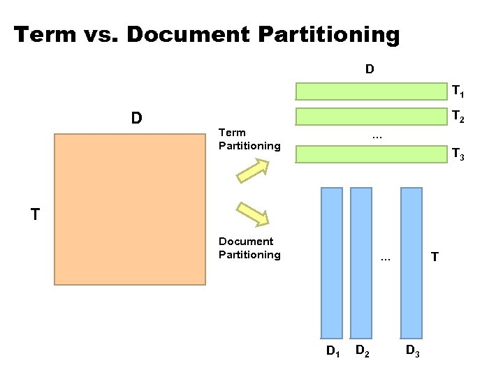Term vs. Document Partitioning D T 1 D T 2 Term Partitioning … T 3 T Document Partitioning T … D 1 D 2 D 3

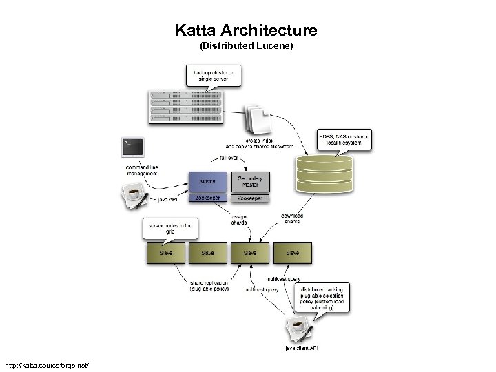Katta Architecture (Distributed Lucene) http: //katta. sourceforge. net/