Industrial Automation Industrielle Automation set point controller

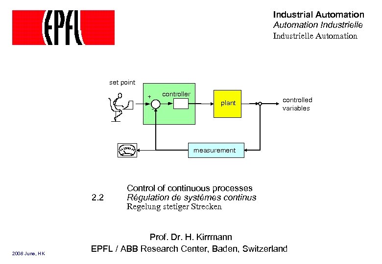Industrial Automation Industrielle Automation set point controller + - plant controlled variables measurement 2. 2 2008 June, HK Control of continuous processes Régulation de systèmes continus Regelung stetiger Strecken Prof. Dr. H. Kirrmann EPFL / ABB Research Center, Baden, Switzerland

2. 2 Control 2. 1 Instrumentation 2. 2 Control 2. 2. 1 Plant modeling 2. 2. 2 Controllers 2. 2. 2. 1 On/Off (two-point) controller 2. 2 PID controller 2. 2. 2. 3 Nested Controllers 2. 3 Programmable Logic Controllers Industrial Automation 2 2. 2 Control

Motivation This is an intuitive introduction to automatic control intended for students who did not enjoy automatic control courses as a preparation for the PLC programming. For a theoretical development, the courses of Prof. Longchamp and Prof. Bonvin are highly recommended. First, modeling of plants is introduced. Then, the two most popular controllers in industry are presented: - the two-point controller - the PID controller Finally, nested controllers are introduced. Industrial Automation 3 2. 2 Control

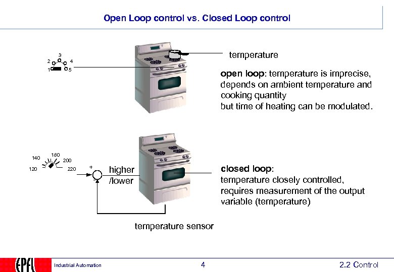Open Loop control vs. Closed Loop control temperature 3 2 1 140 120 4 5 open loop: temperature is imprecise, depends on ambient temperature and cooking quantity but time of heating can be modulated. 180 200 220 + - closed loop: temperature closely controlled, requires measurement of the output variable (temperature) higher /lower temperature sensor Industrial Automation 4 2. 2 Control

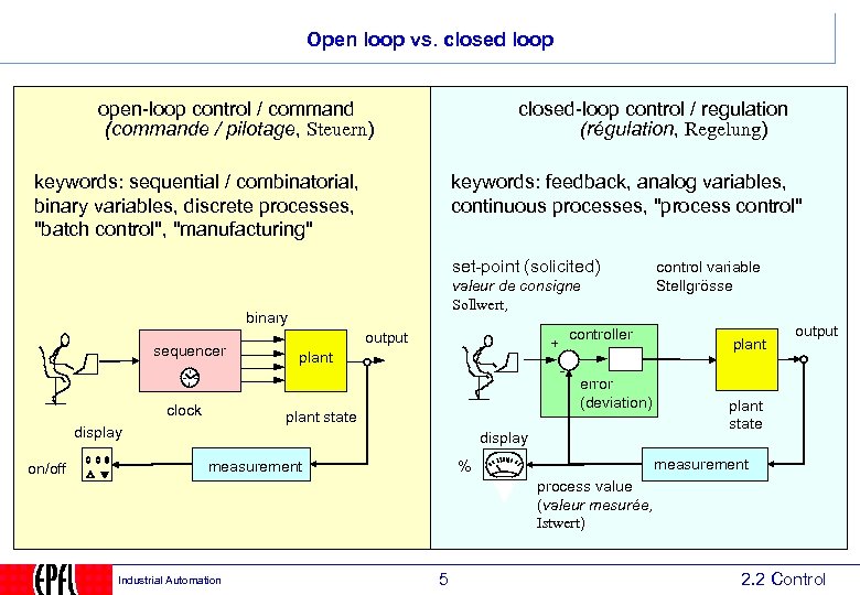Open loop vs. closed loop open-loop control / command (commande / pilotage, Steuern) closed-loop control / regulation (régulation, Regelung) keywords: sequential / combinatorial, binary variables, discrete processes, "batch control", "manufacturing" keywords: feedback, analog variables, continuous processes, "process control" set-point (solicited) valeur de consigne Sollwert, binary sequencer clock controller + plant - plant state display on/off output error (deviation) display measurement control variable Stellgrösse plant output plant state measurement % process value (valeur mesurée, Istwert) Industrial Automation 5 2. 2 Control

2. 2. 1 Plant Modeling 2. 1 Instrumentation 2. 2 Control 2. 2. 1 Plant modeling 2. 2. 2 Controllers 2. 2. 2. 1 On/Off (two-point) controller 2. 2 PID controller 2. 2. 2. 3 Nested Controllers 2. 3 Programmable Logic Controllers Industrial Automation 6 2. 2 Control

Modeling The first step in analysis of control systems is to know the plant to be controlled. The second step is define a controller that meets physical and economical requirements Knowing means express the plant’s behavior in a mathematical way, generally as a system of differential equations, - by analyzing the physical principles (requires that all elements are precisely known) - by identifying the plant’s parameters by analyzing its behavior (output) in response to an input change. Industrial Automation 7 2. 2 Control

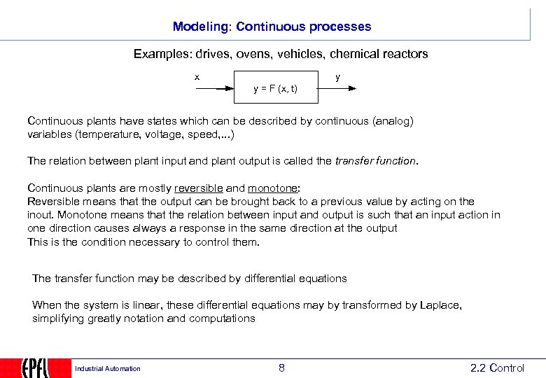Modeling: Continuous processes Examples: drives, ovens, vehicles, chemical reactors x y y = F (x, t) Continuous plants have states which can be described by continuous (analog) variables (temperature, voltage, speed, . . . ) The relation between plant input and plant output is called the transfer function. Continuous plants are mostly reversible and monotone: Reversible means that the output can be brought back to a previous value by acting on the inout. Monotone means that the relation between input and output is such that an input action in one direction causes always a response in the same direction at the output This is the condition necessary to control them. The transfer function may be described by differential equations When the system is linear, these differential equations may by transformed by Laplace, simplifying greatly notation and computations Industrial Automation 8 2. 2 Control

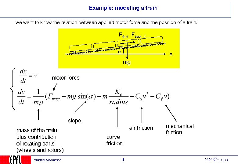Example: modeling a train we want to know the relation between applied motor force and the position of a train. Ffrict Ftract x mg motor force slope mass of the train plus contribution of rotating parts (wheels and rotors) Industrial Automation air friction curve friction 9 mechanical friction 2. 2 Control

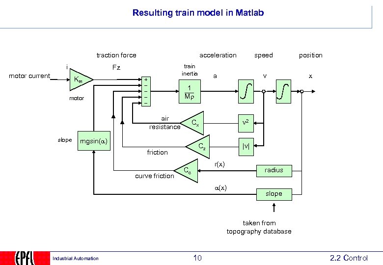Resulting train model in Matlab traction force i acceleration train inertia Fz motor current Km v a position x 1 Mr motor air resistance slope speed Cx mgsin( ) Cz friction curve friction v 2 |v| r(x) Cc (x) radius slope taken from topography database Industrial Automation 10 2. 2 Control

Thermal (solid) and electrical model: conductivity q = heat flow [J/s = W] T = temperature [K] T 2 R = thermal resistance [K/W] T 1 q= k = thermal conductivity [J/m/K] (T 2 – T 1) = (T 2 – T 1) R k. A d A = surface [m 2] R= d = distance [m] A I = current [A] U = voltage [V] R = resistance [Ω] d U 2 U 1 i i= A d (U 2 – U 1) 11 = (U 2 – U 1) R R=ρ ρ = resistivity [Vm] Industrial Automation d k. A A ρd d A 2. 2 Control

Thermal (solid) and electrical model: capacity q = heat flow [J/s = W] T = temperature [K] T C = thermal capacity [J/K] q=C Cm = thermal specific [J/K/kg] d. T C= dt Cm ρV = Cm ρAd A = surface [m 2] d = distance [m] ρ = density A d [kg/m 3] I = current [A] U = voltage [V] U i=C i dt C = capacity [F] ε = dielectric constant [F/m] Industrial Automation d. U A C=ε A d d 12 2. 2 Control

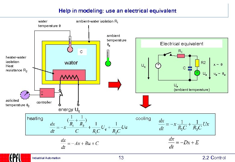Help in modeling: use an electrical equivalent water temperature ambient-water isolation R 1 ambient temperature a Electrical equivalent R 1 C heater-water isolation Heat resistance R 2 water Uq R 2 C Ua x~ ua ~ a Ua (ambient temperature) solicited temperature 2 controller energy Uq heating Industrial Automation cooling 13 2. 2 Control

2. 2. 2 Controllers 2. 1 Instrumentation 2. 2 Control 2. 2. 1 Plant modeling 2. 2. 2 Controllers 2. 2. 2. 1 On/Off (two-point) controller 2. 2 PID controller 2. 2. 2. 3 Nested Controllers 2. 3 Programmable Logic Controllers Industrial Automation 14 2. 2 Control

Controllers Once the plant is known, a controller can be designed to control its output. If the plant would be perfectly known, no regulation would be needed. In practice, the plant’s parameters vary ( e. g. number of passengers in a train), the plant is subject to disturbances (wind, slope) The controller needs measuring through sensors the plant’s state and possibly the disturbances. In a general model, the desired behaviour of the plant is just a disturbance. The controller follows certain quality laws, primarily to stabilize the output within useful time, not overshoot, minimize energy consumption, etc…. . Industrial Automation 15 2. 2 Control

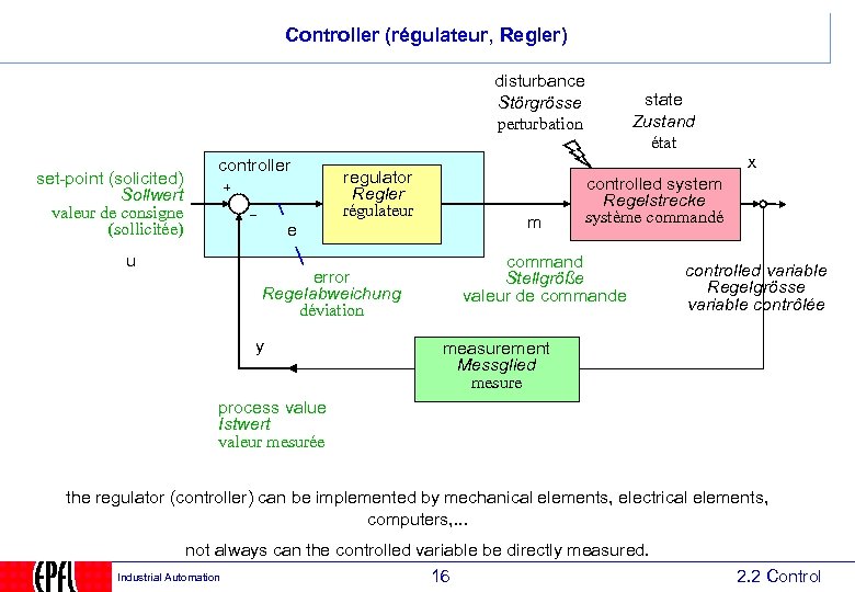Controller (régulateur, Regler) disturbance Störgrösse perturbation set-point (solicited) Sollwert valeur de consigne (sollicitée) u controller regulator Regler régulateur e error Regelabweichung déviation y state Zustand état x m controlled system Regelstrecke système commandé command Stellgröße valeur de commande controlled variable Regelgrösse variable contrôlée measurement Messglied mesure process value Istwert valeur mesurée the regulator (controller) can be implemented by mechanical elements, electrical elements, computers, . . . not always can the controlled variable be directly measured. Industrial Automation 16 2. 2 Control

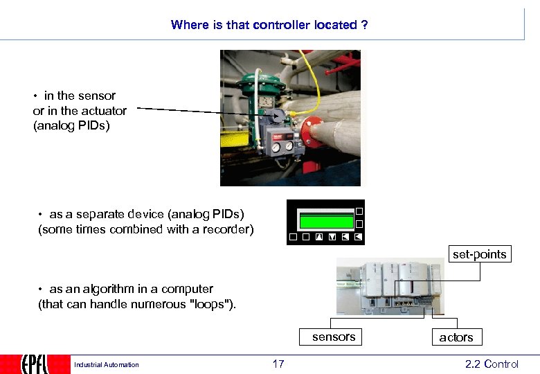Where is that controller located ? • in the sensor or in the actuator (analog PIDs) • as a separate device (analog PIDs) (some times combined with a recorder) set-points • as an algorithm in a computer (that can handle numerous "loops"). sensors Industrial Automation 17 actors 2. 2 Control

2. 2. 2. 1 On/Off (two-point) controller 2. 1 Instrumentation 2. 2 Control 2. 2. 1 Plant modeling 2. 2. 2 Controllers 2. 2. 2. 1 On/Off (two-point) controller 2. 2 PID controller 2. 2. 2. 3 Nested Controllers 2. 3 Programmable Logic Controllers Industrial Automation 18 2. 2 Control

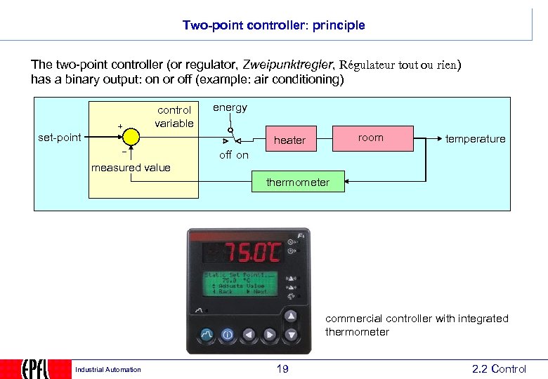Two-point controller: principle The two-point controller (or regulator, Zweipunktregler, Régulateur tout ou rien) has a binary output: on or off (example: air conditioning) control variable energy set-point room heater temperature off on measured value thermometer commercial controller with integrated thermometer Industrial Automation 19 2. 2 Control

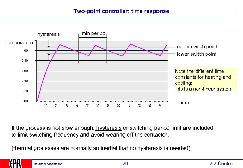Two-point controller: time response min period hysteresis temperature upper switch point lower switch point 1. 00 0. 80 Note the different time constants for heating and cooling: this is a non-linear system 0. 60 0. 40 0. 20 97 89 81 73 65 57 49 41 33 25 17 9 1 0. 00 time If the process is not slow enough, hysteresis or switching period limit are included to limit switching frequency and avoid wearing off the contactor. (thermal processes are normally so inertial that no hysteresis is needed) Industrial Automation 20 2. 2 Control

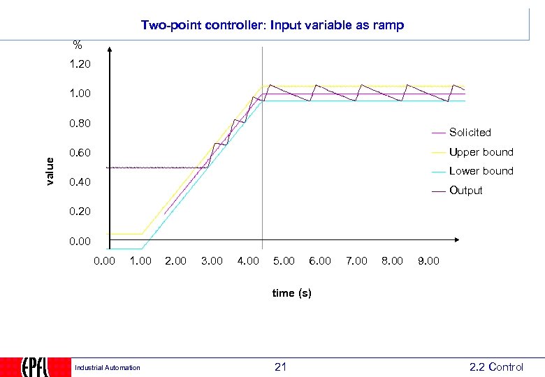Two-point controller: Input variable as ramp % 1. 20 1. 00 value 0. 80 Solicited Upper bound 0. 60 Lower bound 0. 40 Output 0. 20 0. 00 1. 00 2. 00 3. 00 4. 00 5. 00 6. 00 7. 00 8. 00 9. 00 time (s) Industrial Automation 21 2. 2 Control

2. 2 PID Controller 2. 1 Instrumentation 2. 2 Control 2. 2. 1 Plant modeling 2. 2. 2 Controllers 2. 2. 2. 1 On/Off (two-point) controller 2. 2 PID controller 2. 2. 2. 3 Nested Controllers 2. 3 Programmable Logic Controllers Industrial Automation 22 2. 2 Control

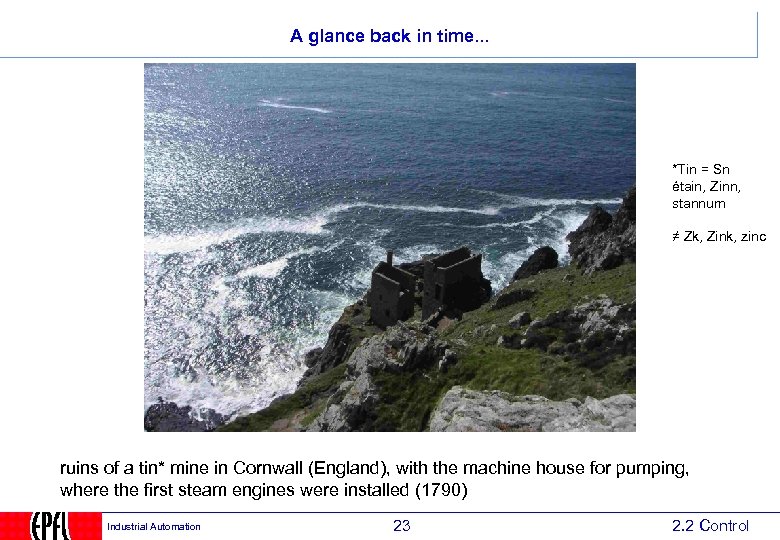A glance back in time. . . *Tin = Sn étain, Zinn, stannum ≠ Zk, Zink, zinc ruins of a tin* mine in Cornwall (England), with the machine house for pumping, where the first steam engines were installed (1790) Industrial Automation 23 2. 2 Control

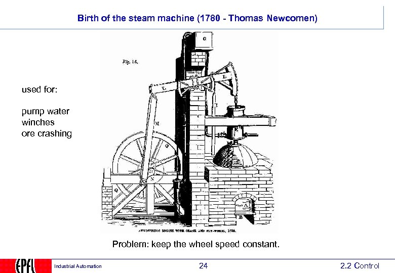Birth of the steam machine (1780 - Thomas Newcomen) used for: pump water winches ore crashing Problem: keep the wheel speed constant. Industrial Automation 24 2. 2 Control

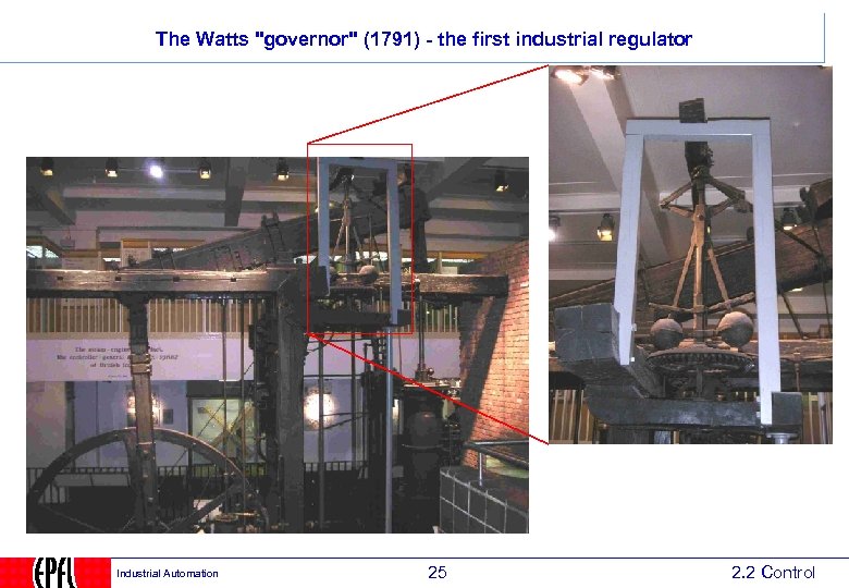The Watts "governor" (1791) - the first industrial regulator Industrial Automation 25 2. 2 Control

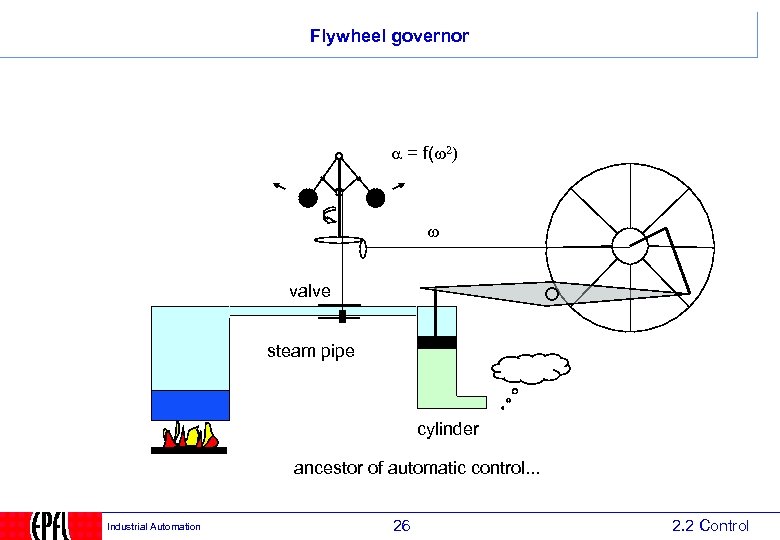Flywheel governor = f(w 2) w valve steam pipe cylinder ancestor of automatic control. . . Industrial Automation 26 2. 2 Control

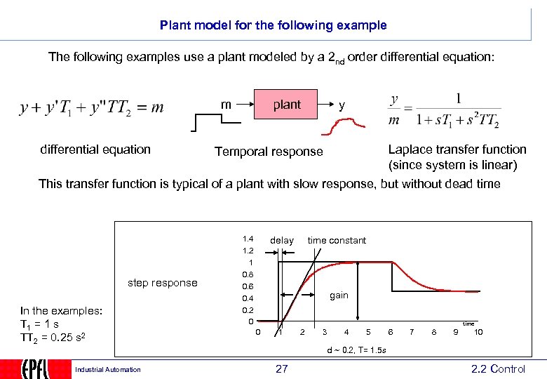Plant model for the following example The following examples use a plant modeled by a 2 nd order differential equation: m differential equation plant y Laplace transfer function (since system is linear) Temporal response This transfer function is typical of a plant with slow response, but without dead time 1. 4 delay time constant 1. 2 1 step response In the examples: T 1 = 1 s TT 2 = 0. 25 s 2 Industrial Automation 0. 8 0. 6 0. 4 gain 0. 2 0 time 0 1 2 3 4 5 6 7 8 9 10 d ~ 0. 2, T= 1. 5 s 27 2. 2 Control

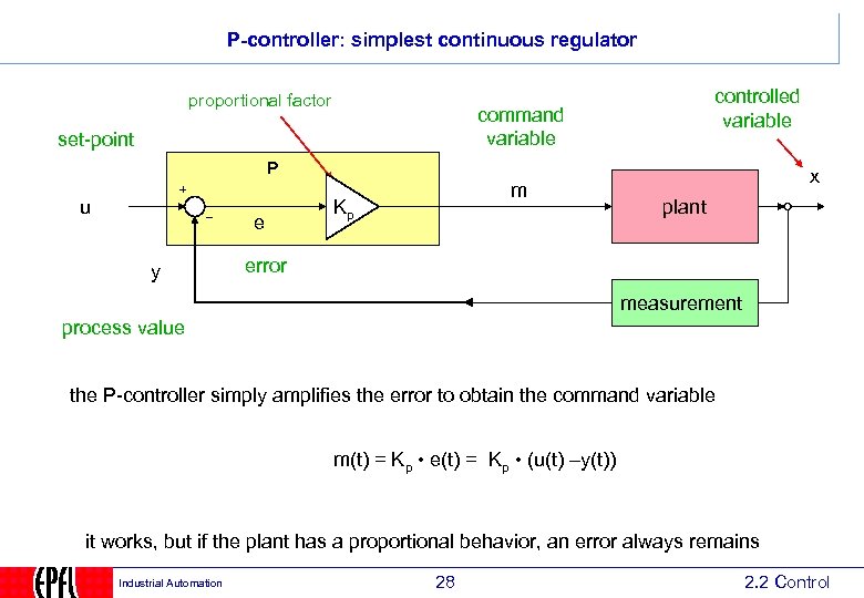P-controller: simplest continuous regulator proportional factor controlled variable command variable set-point P u e y m Kp x plant error measurement process value the P-controller simply amplifies the error to obtain the command variable m(t) = Kp • e(t) = Kp • (u(t) –y(t)) it works, but if the plant has a proportional behavior, an error always remains Industrial Automation 28 2. 2 Control

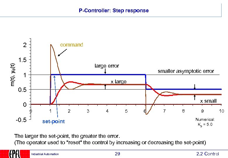P-Controller: Step response m(t), y 0(t) 2 command 1. 5 large error smaller asymptotic error 1 x large 0. 5 x small 0 0 -0. 5 1 2 3 4 5 6 7 8 9 10 Numerical: Kp = 5. 0 set-point The larger the set-point, the greater the error. (The operator used to "reset" the control by increasing or decreasing the set-point) Industrial Automation 29 2. 2 Control

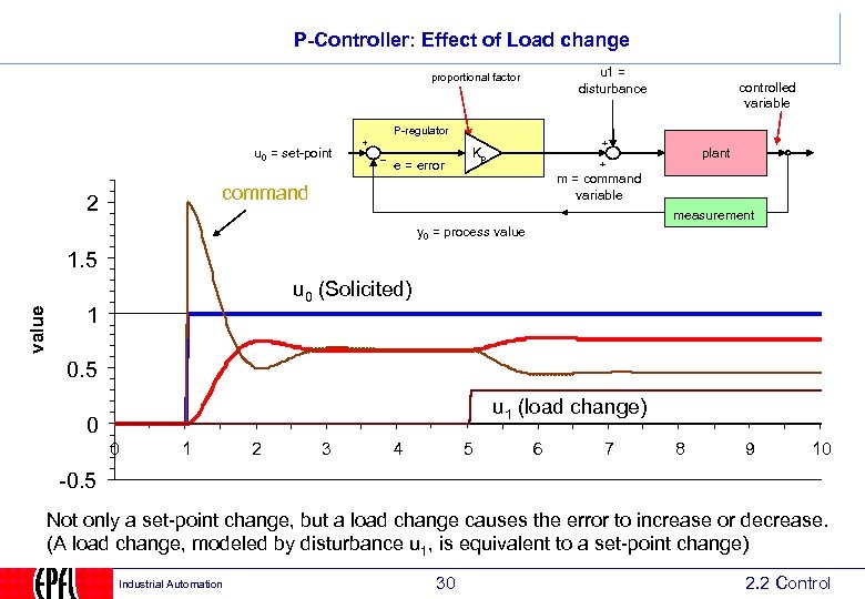P-Controller: Effect of Load change u 1 = disturbance proportional factor controlled variable P-regulator u 0 = set-point e = error Kp plant m = command variable command 2 measurement y 0 = process value 1. 5 u 0 (Solicited) 1 0. 5 u 1 (load change) 0 0 1 2 3 4 5 6 7 8 9 10 -0. 5 Not only a set-point change, but a load change causes the error to increase or decrease. (A load change, modeled by disturbance u 1, is equivalent to a set-point change) Industrial Automation 30 2. 2 Control

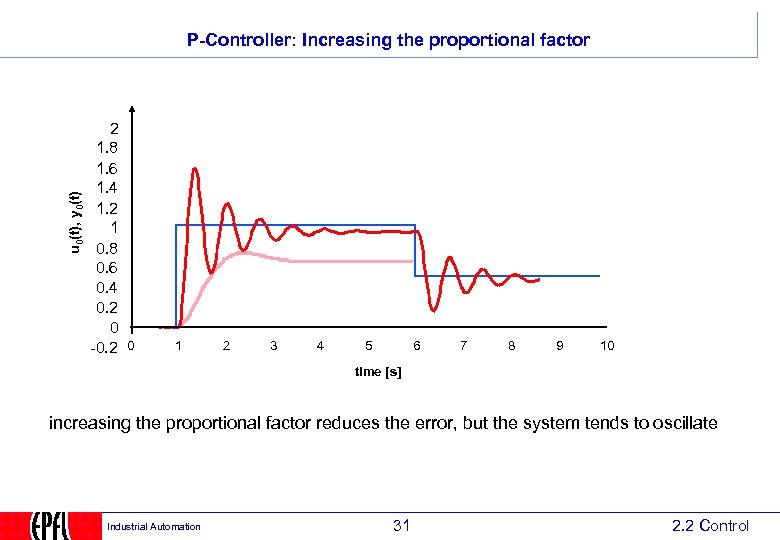u 0(t), y 0(t) P-Controller: Increasing the proportional factor 2 1. 8 1. 6 1. 4 1. 2 1 0. 8 0. 6 0. 4 0. 2 0 -0. 2 0 1 2 3 4 5 6 7 8 9 10 time [s] increasing the proportional factor reduces the error, but the system tends to oscillate Industrial Automation 31 2. 2 Control

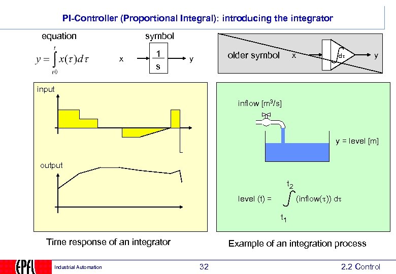PI-Controller (Proportional Integral): introducing the integrator equation symbol x 1 s older symbol y x dt y input inflow [m 3/s] y = level [m] output t 2 level (t) = (inflow(t)) dt t 1 Time response of an integrator Industrial Automation Example of an integration process 32 2. 2 Control

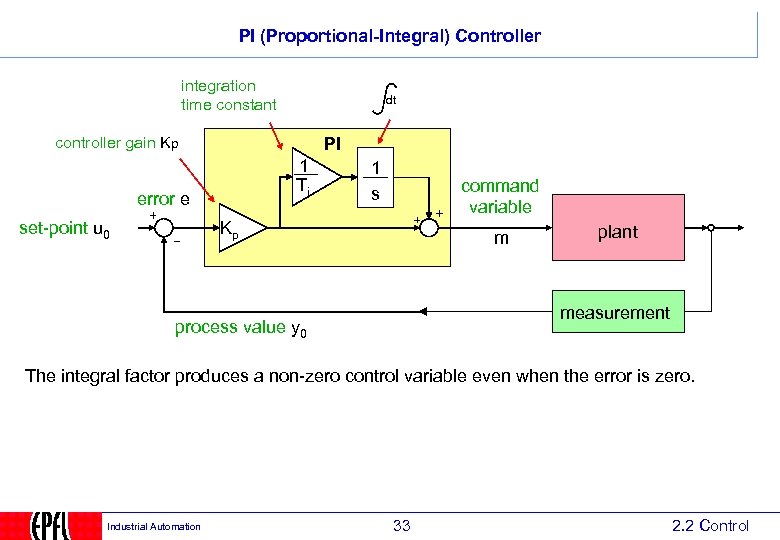PI (Proportional-Integral) Controller integration time constant dt controller gain Kp PI 1 Ti error e set-point u 0 1 s command variable Kp m plant measurement process value y 0 The integral factor produces a non-zero control variable even when the error is zero. Industrial Automation 33 2. 2 Control

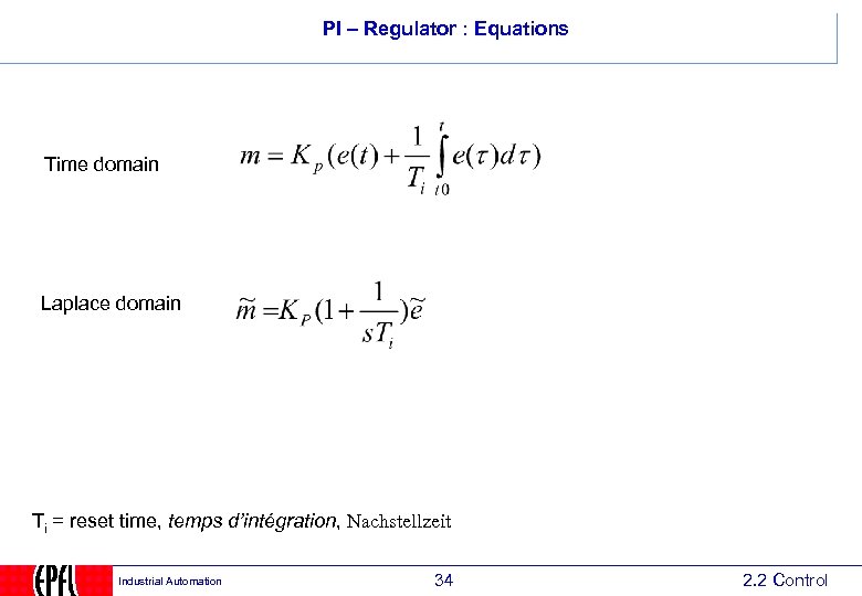PI – Regulator : Equations Time domain Laplace domain Ti = reset time, temps d’intégration, Nachstellzeit Industrial Automation 34 2. 2 Control

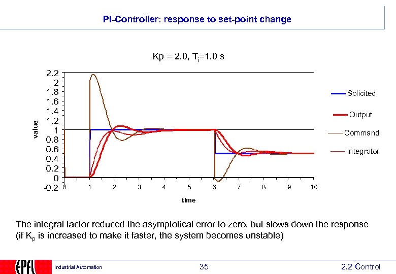PI-Controller: response to set-point change value Kp = 2, 0, Ti=1, 0 s 2. 2 2 1. 8 1. 6 1. 4 1. 2 1 0. 8 0. 6 0. 4 0. 2 0 -0. 2 Solicited Output Command Integrator 0 1 2 3 4 5 6 7 8 9 10 time The integral factor reduced the asymptotical error to zero, but slows down the response (if Kp is increased to make it faster, the system becomes unstable) Industrial Automation 35 2. 2 Control

PD controller Basic idea of the PD regulator: take into account not only the value of the error, but the rate at which the error changes. Example: when parking a car in front of a wall, the driver not only looks at the distance to the wall, but also at the speed at which the car approaches the wall. Industrial Automation 36 2. 2 Control

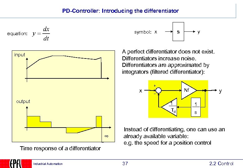PD-Controller: Introducing the differentiator s symbol: x equation: y A perfect differentiator does not exist. Differentiators increase noise. Differentiators are approximated by integrators (filtered differentiator): input Nf x output 1 Td ∞ Time response of a differentiator Industrial Automation y 1 s Instead of differentiating, one can use an already available variable: e. g. the speed for a position control 37 2. 2 Control

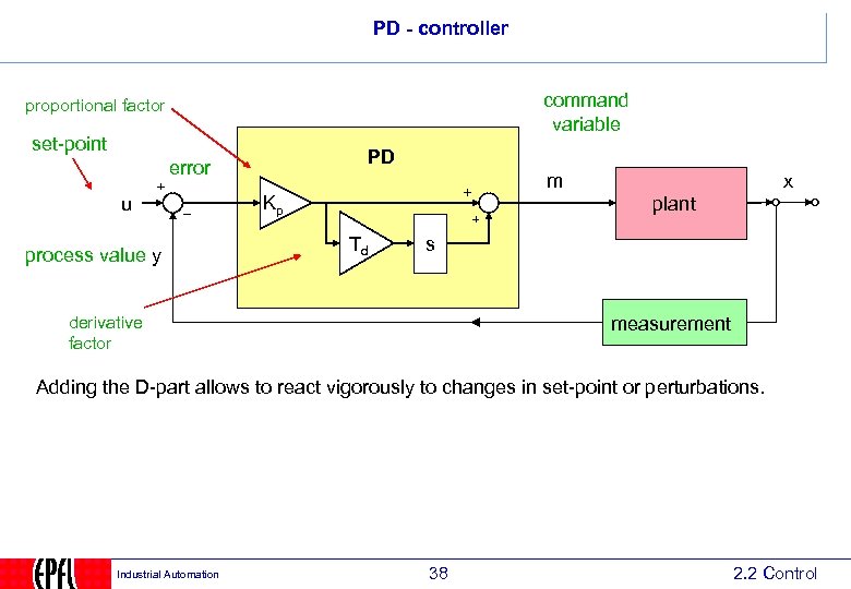PD - controller command variable proportional factor set-point PD error u process value y m Kp x plant Td s derivative factor measurement Adding the D-part allows to react vigorously to changes in set-point or perturbations. Industrial Automation 38 2. 2 Control

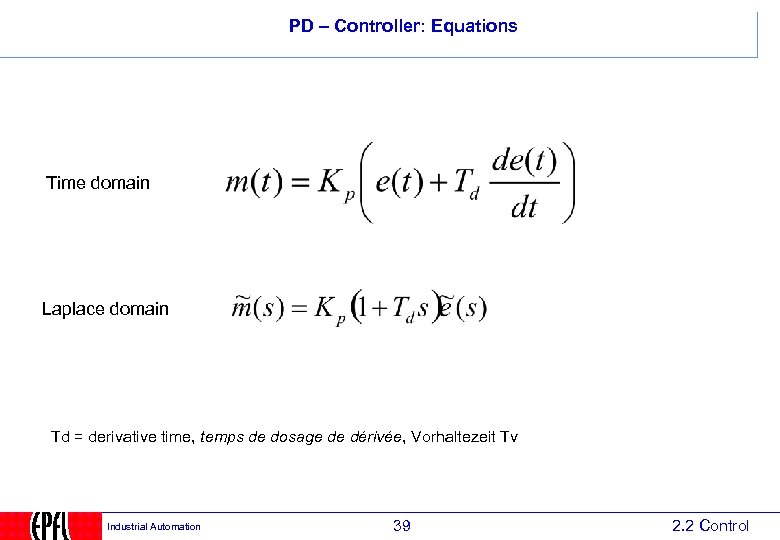PD – Controller: Equations Time domain Laplace domain Td = derivative time, temps de dosage de dérivée, Vorhaltezeit Tv Industrial Automation 39 2. 2 Control

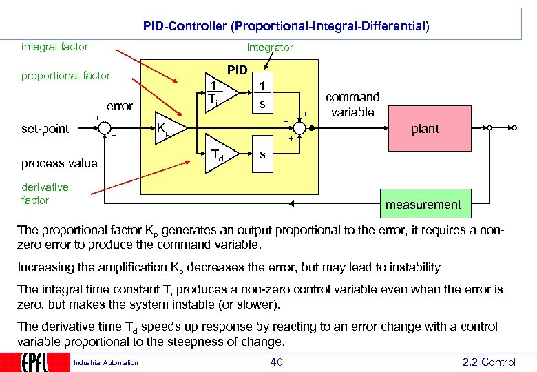PID-Controller (Proportional-Integral-Differential) integral factor integrator PID proportional factor 1 Ti error 1 s command variable Kp set-point process value plant Td s derivative factor measurement The proportional factor Kp generates an output proportional to the error, it requires a nonzero error to produce the command variable. Increasing the amplification Kp decreases the error, but may lead to instability The integral time constant Ti produces a non-zero control variable even when the error is zero, but makes the system instable (or slower). The derivative time Td speeds up response by reacting to an error change with a control variable proportional to the steepness of change. Industrial Automation 40 2. 2 Control

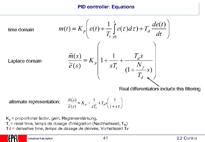PID controller: Equations time domain Laplace domain Real differentiators include this filtering alternate representation: Kp = proportional factor, gain, Reglerverstärkung, Ti = reset time, temps de dosage d’intégration (Nachhaltezeit, TN) Td = derivative time, temps de dosage de dérivée, Vorhaltezeit Tv Industrial Automation 41 2. 2 Control

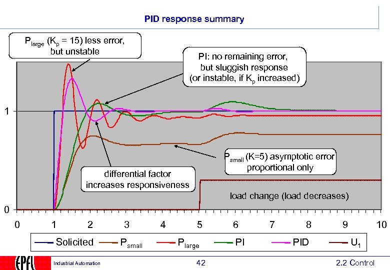PID response summary Plarge (Kp = 15) less error, but unstable PI: no remaining error, but sluggish response (or instable, if Kp increased) 1 Psmall (K=5) asymptotic error proportional only differential factor increases responsiveness load change (load decreases) 0 0 1 2 Solicited Industrial Automation 3 Psmall 4 5 Plarge 42 6 PI 7 8 PID 9 10 U 1 2. 2 Control

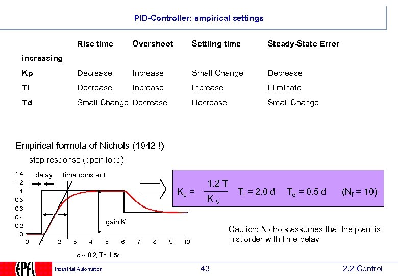PID-Controller: empirical settings Rise time Overshoot Settling time Steady-State Error Kp Decrease Increase Small Change Decrease Ti Decrease Increase Eliminate Td Small Change Decrease Small Change increasing Empirical formula of Nichols (1942 !) step response (open loop) 1. 4 delay time constant 1. 2 1 Kp = 0. 8 0. 6 0. 4 1. 2 T KV gain K 0. 2 0 0 1 2 3 4 5 6 7 8 9 Ti = 2. 0 d Td = 0. 5 d (Nf = 10) Caution: Nichols assumes that the plant is first order with time delay 10 d ~ 0. 2, T= 1. 5 s Industrial Automation 43 2. 2 Control

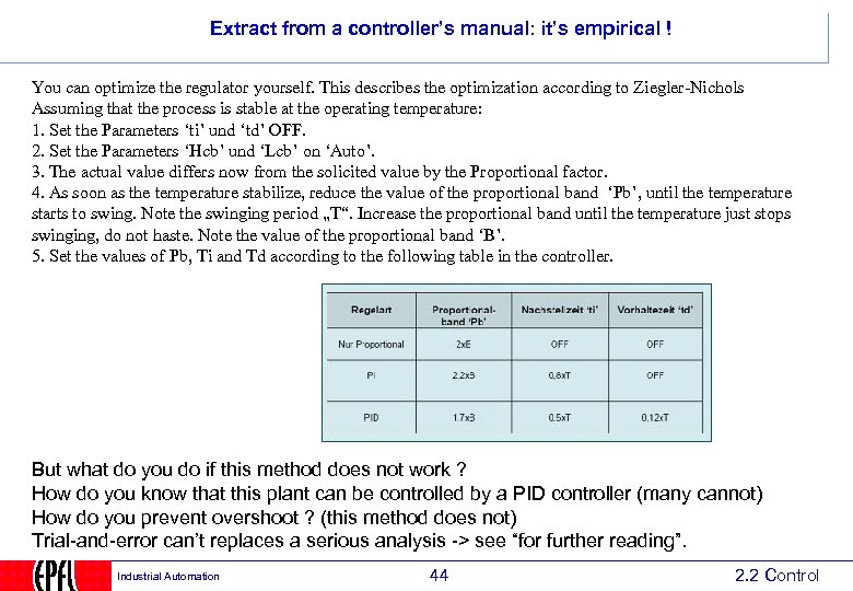Extract from a controller’s manual: it’s empirical ! You can optimize the regulator yourself. This describes the optimization according to Ziegler-Nichols Assuming that the process is stable at the operating temperature: 1. Set the Parameters ‘ti’ und ‘td’ OFF. 2. Set the Parameters ‘Hcb’ und ‘Lcb’ on ‘Auto’. 3. The actual value differs now from the solicited value by the Proportional factor. 4. As soon as the temperature stabilize, reduce the value of the proportional band ‘Pb’, until the temperature starts to swing. Note the swinging period „T“. Increase the proportional band until the temperature just stops swinging, do not haste. Note the value of the proportional band ‘B’. 5. Set the values of Pb, Ti and Td according to the following table in the controller. But what do you do if this method does not work ? How do you know that this plant can be controlled by a PID controller (many cannot) How do you prevent overshoot ? (this method does not) Trial-and-error can’t replaces a serious analysis -> see “for further reading”. Industrial Automation 44 2. 2 Control

2. 2. 2. 3 Nested controllers 2. 1 Instrumentation 2. 2 Control 2. 2. 1 Plant modeling 2. 2. 2 Controllers 2. 2. 2. 1 On/Off (two-point) controller 2. 2 PID controller 2. 2. 2. 3 Nested Controllers 2. 3 Programmable Logic Controllers Industrial Automation 45 2. 2 Control

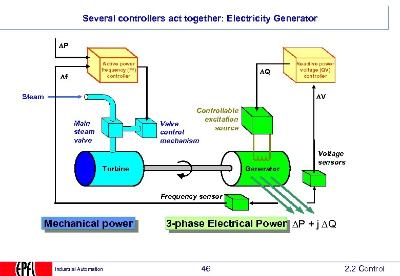Several controllers act together: Electricity Generator P Active power frequency (Pf) controller f Q Reactive power voltage (QV) controller V Steam Controllable excitation source Main steam valve Valve control mechanism Turbine Generator Voltage sensors Frequency sensor Mechanical power Industrial Automation 3 -phase Electrical Power DP + j DQ 46 2. 2 Control

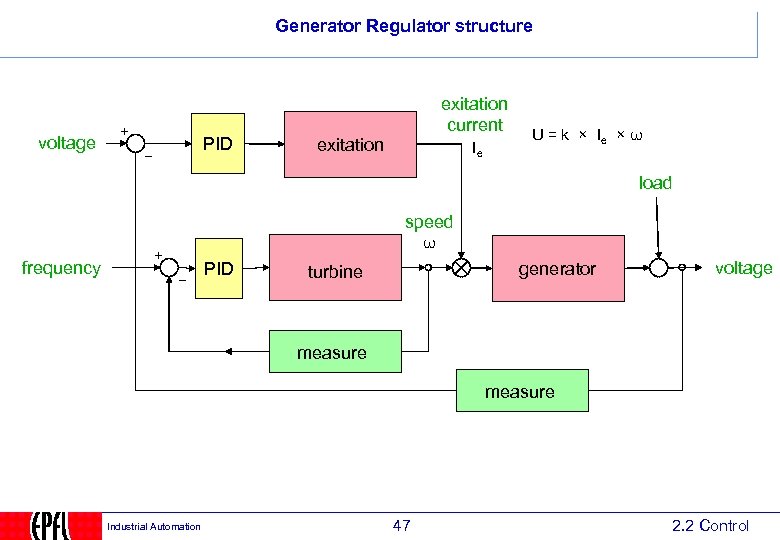Generator Regulator structure voltage PID exitation current exitation Ie U = k × Ie × ω load speed ω frequency PID generator turbine voltage measure Industrial Automation 47 2. 2 Control

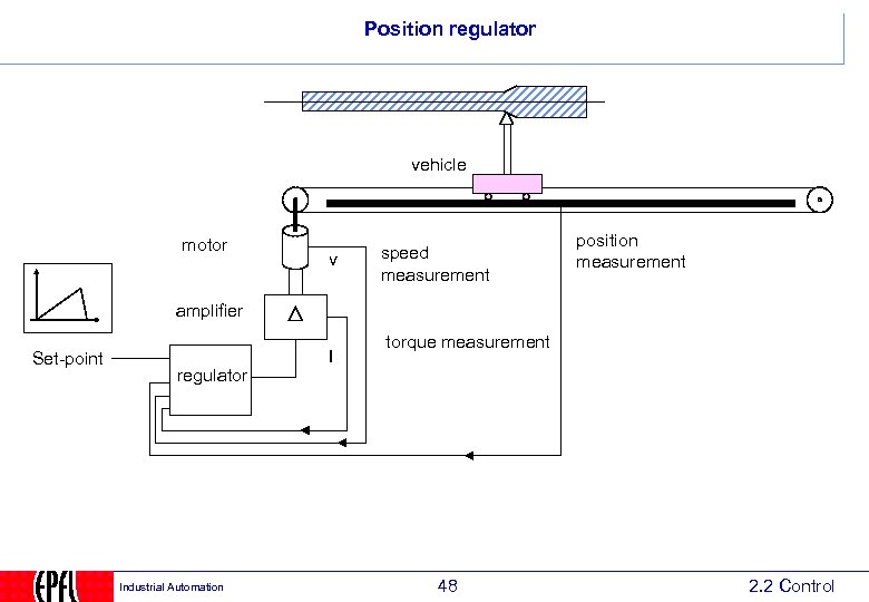Position regulator vehicle motor v speed measurement position measurement amplifier Set-point regulator Industrial Automation I torque measurement 48 2. 2 Control

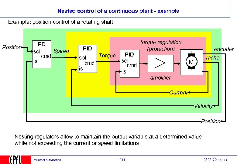Nested control of a continuous plant - example Example: position control of a rotating shaft Position PD Speed sol cmd is PID Torque sol cmd is PID sol cmd is torque regulation (protection) encoder tacho M amplifier Current Velocity Position Nesting regulators allow to maintain the output variable at a determined value while not exceeding the current or speed limitations Industrial Automation 49 2. 2 Control

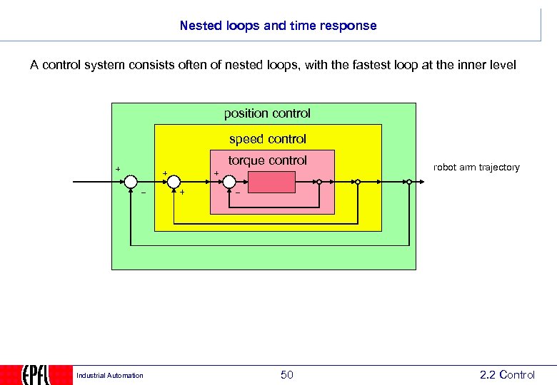Nested loops and time response A control system consists often of nested loops, with the fastest loop at the inner level position control speed control torque control Industrial Automation 50 robot arm trajectory 2. 2 Control

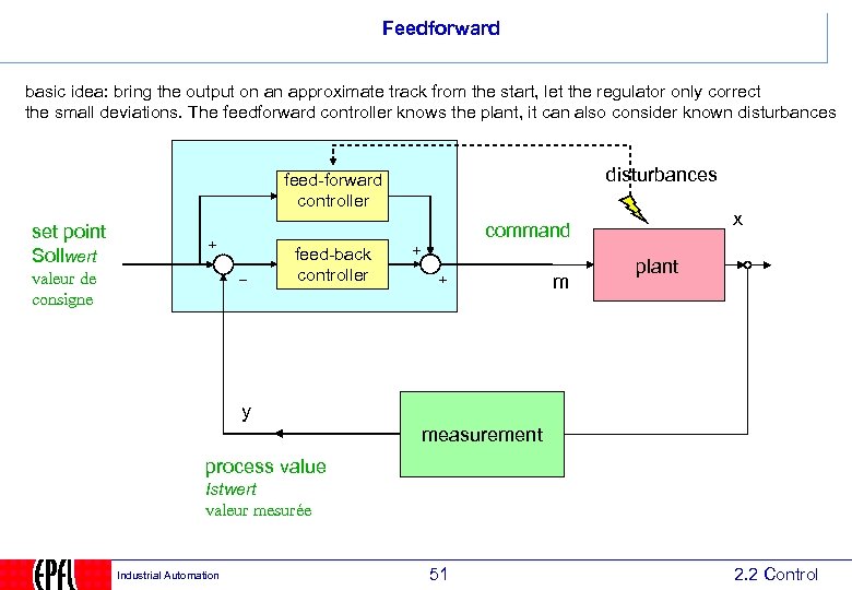Feedforward basic idea: bring the output on an approximate track from the start, let the regulator only correct the small deviations. The feedforward controller knows the plant, it can also consider known disturbances feed-forward controller x command set point Sollwert feed-back controller valeur de consigne m plant y measurement process value Istwert valeur mesurée Industrial Automation 51 2. 2 Control

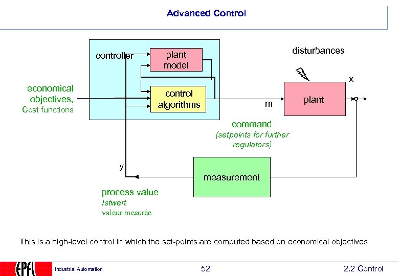Advanced Control disturbances plant model controller x economical objectives, control algorithms Cost functions m plant command (setpoints for further regulators) y measurement process value Istwert valeur mesurée This is a high-level control in which the set-points are computed based on economical objectives Industrial Automation 52 2. 2 Control

Assessment How does a two-point regulator works ? How is the a wear-out of the contacts prevented ? How does a PID regulator works ? What is the influence of the different parameters of a PID ? Is a PID controller required for a position control system (motor moves a vehicle) Explain the relation between nesting control loops and their real-time response What is feed-forward control ? Industrial Automation 53 2. 2 Control

To probe further Courses of Prof. Longchamp and Prof. Bonvin "Computer Systems for Automation and Control", Gustaf Olsson, Gianguido Piani, Lund Institute of Technology “Modern Control Systems”, R. Dorf, Addison Wesley Industrial Automation 54 2. 2 Control