 INC 551 Artificial Intelligence Lecture 8 Models of Uncertainty
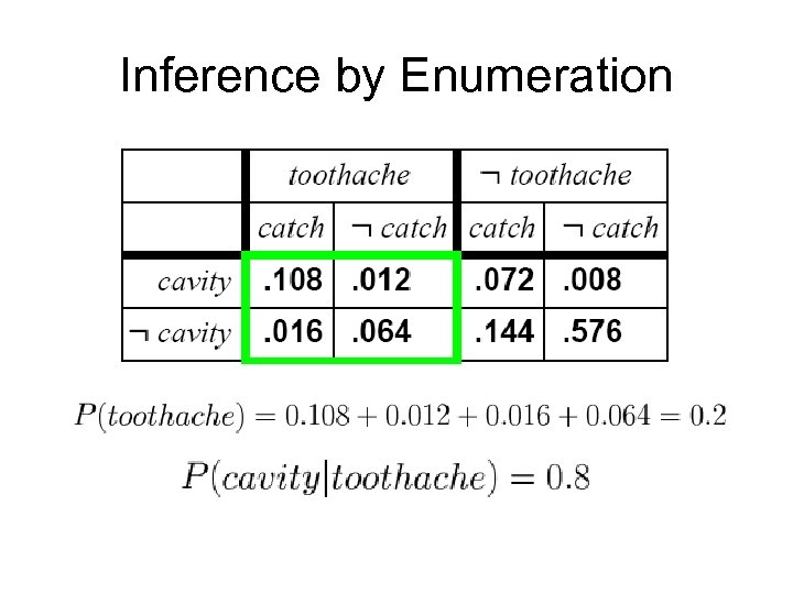 Inference by Enumeration
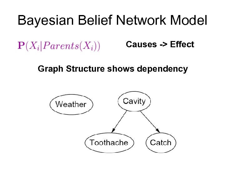 Bayesian Belief Network Model Causes -> Effect Graph Structure shows dependency
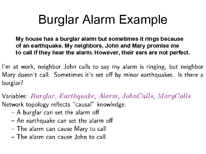 Burglar Alarm Example My house has a burglar alarm but sometimes it rings because of an earthquake. My neighbors, John and Mary promise me to call if they hear the alarm. However, their ears are not perfect.
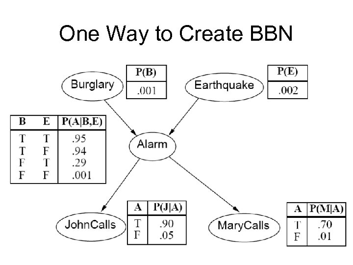 One Way to Create BBN
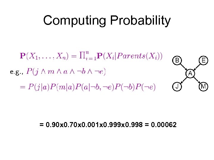 Computing Probability = 0. 90 x 0. 70 x 0. 001 x 0. 999 x 0. 998 = 0. 00062
 BBN Construction There are many ways to construct BBN of a problem because the events depend on each other (related). Therefore, it depends on the order of events that you consider. The most simple is the most compact.
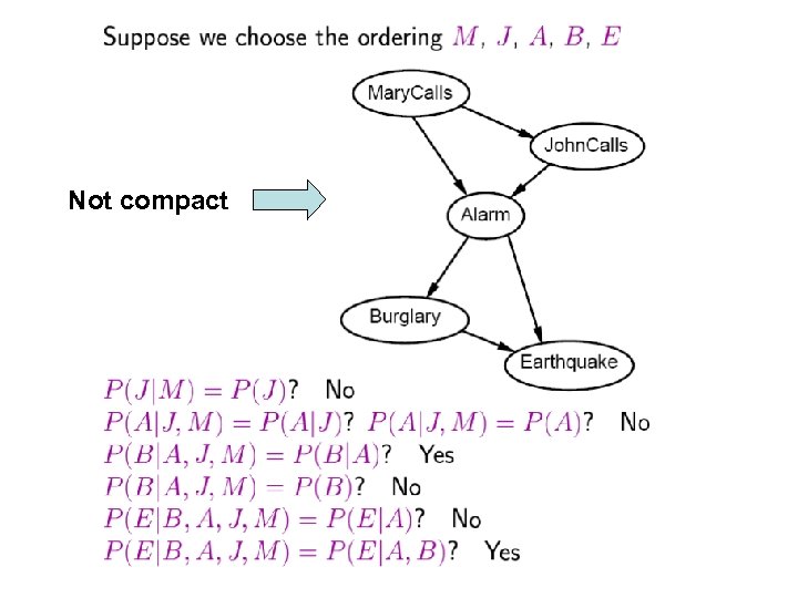 Not compact
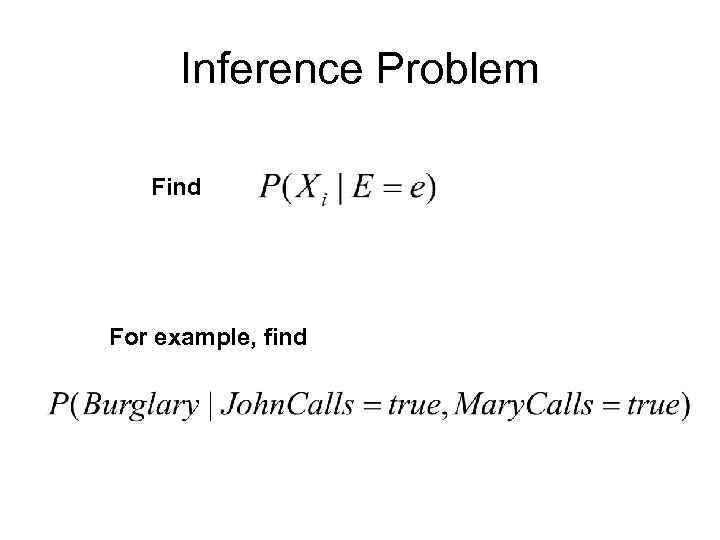 Inference Problem Find For example, find
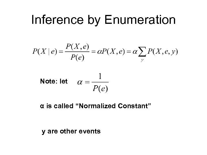 Inference by Enumeration Note: let α is called “Normalized Constant” y are other events
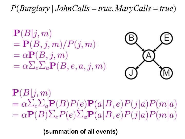 (summation of all events)
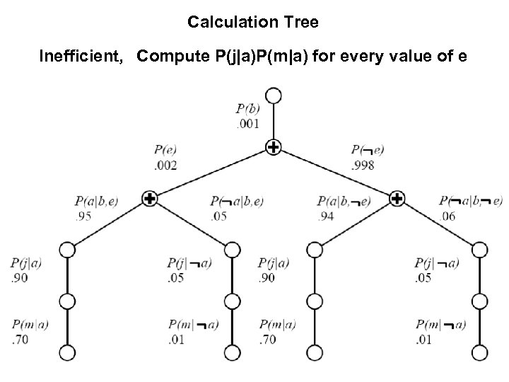 Calculation Tree Inefficient, Compute P(j|a)P(m|a) for every value of e
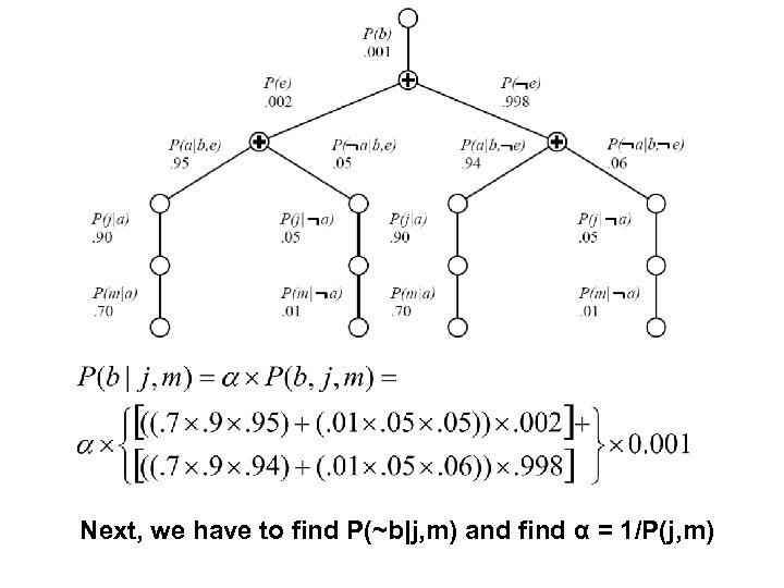 Next, we have to find P(~b|j, m) and find α = 1/P(j, m)
 Approximate Inference Idea: Count from real examples We call this procedure “Sampling” Sampling = get real examples from the world model
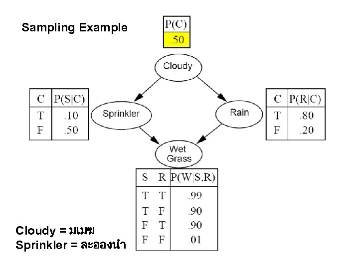 Sampling Example Cloudy = มเมฆ Sprinkler = ละอองนำ
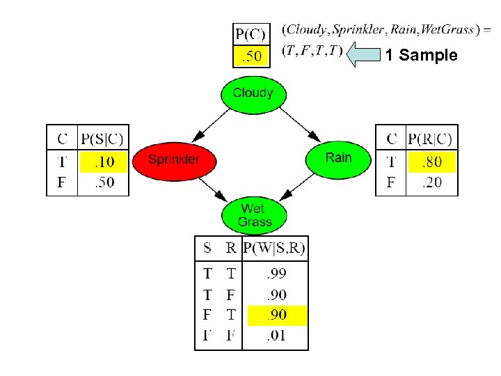 1 Sample
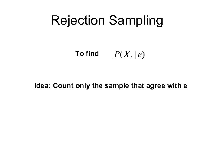 Rejection Sampling To find Idea: Count only the sample that agree with e
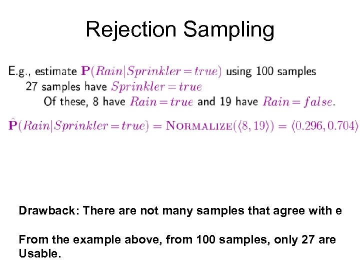 Rejection Sampling Drawback: There are not many samples that agree with e From the example above, from 100 samples, only 27 are Usable.
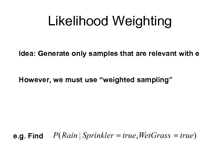 Likelihood Weighting Idea: Generate only samples that are relevant with e However, we must use “weighted sampling” e. g. Find
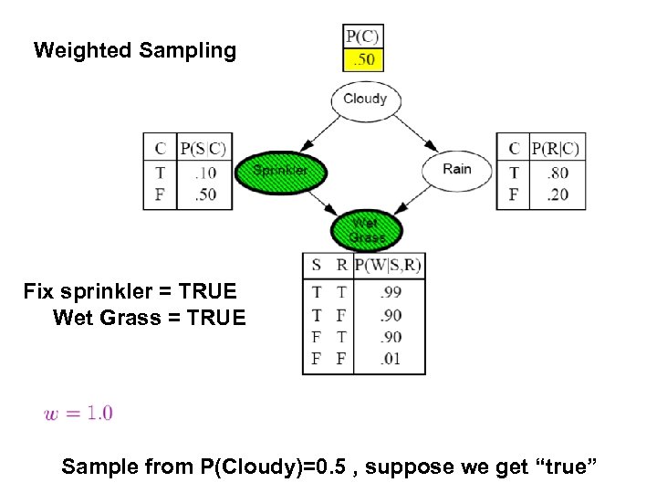 Weighted Sampling Fix sprinkler = TRUE Wet Grass = TRUE Sample from P(Cloudy)=0. 5 , suppose we get “true”
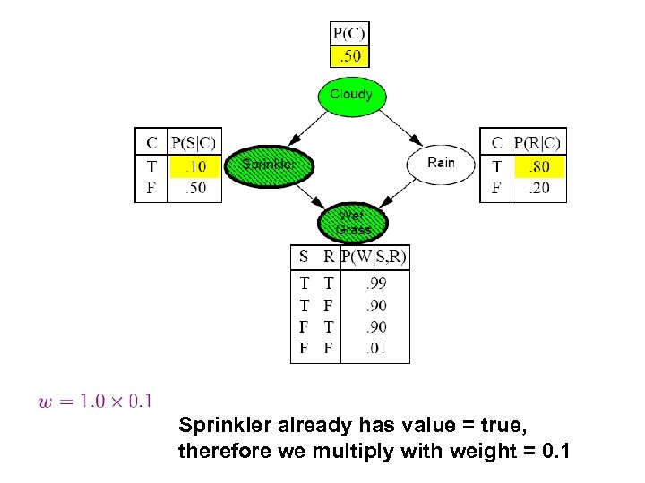 Sprinkler already has value = true, therefore we multiply with weight = 0. 1
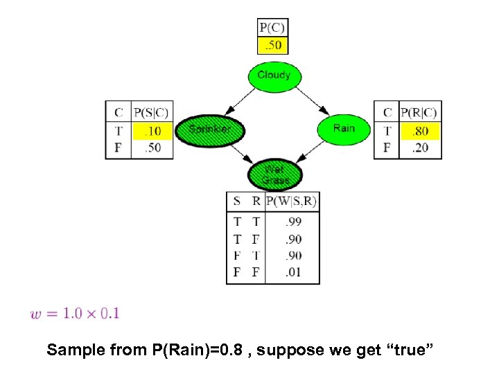 Sample from P(Rain)=0. 8 , suppose we get “true”
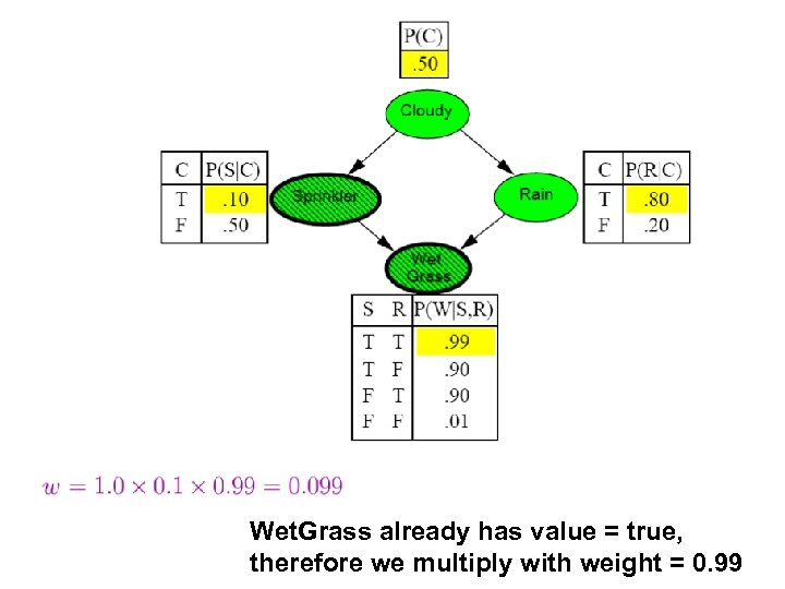 Wet. Grass already has value = true, therefore we multiply with weight = 0. 99
 Finally, we got a sample (t, t, t, t) With weight = 0. 099
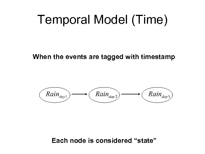 Temporal Model (Time) When the events are tagged with timestamp Each node is considered “state”
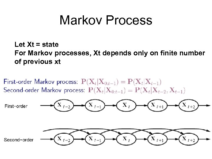 Markov Process Let Xt = state For Markov processes, Xt depends only on finite number of previous xt
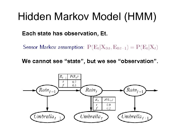 Hidden Markov Model (HMM) Each state has observation, Et. We cannot see “state”, but we see “observation”.