Image segmentation using Eigenvectors Speaker Sameer Agarwal

Image segmentation using Eigenvectors Speaker : Sameer Agarwal Course : Learning and Vision Seminar Date : 09/10/2001

“Theoretically I might say there are 327 brightnesses and nuances of color. Do I have “ 327” No. I have sky, house, and trees. It is impossible to achieve “ 327” as such. And yet even though such droll calculations are possible--- and implied, say, for the house 120, the trees 90 and the sky 117– I should at least have this arrangement and division of the total, and not, say, 127 and 100; or 150 and 177. ” Laws of Organization in Perceptual Forms Max Wertheimer (1923)

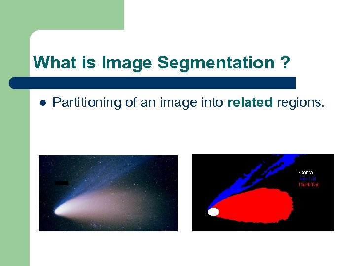What is Image Segmentation ? l Partitioning of an image into related regions.

Why do Image Segmentation ? l l l Image Compression - Identify distinct components within an image and use the most suitable compression algorithm for each component to get a higher compression ratio. Medical Diagnosis - Automatic segmentation of MRI images for identification of cancerous regions Mapping and Measurement - Automatic analysis of remote sensing data from satellites to identify and measure regions of interest. e. g. Petroleum reserves.

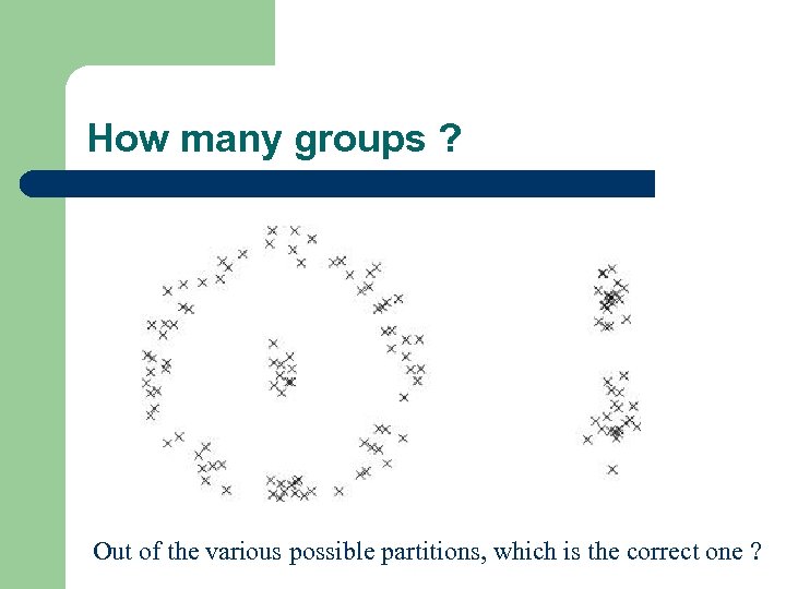How many groups ? Out of the various possible partitions, which is the correct one ?

The bayesian view Given prior knowledge about the structure of the data, choose the partition which is most probable. Problem : How do you specify a prior for knowledge which is composed of knowledge on multiple scales. e. g. – – Coherence Symmetry

A simplementation l l Assume that the image was generated by a mixture of multiple models Segmentation is done in two steps : 1. 2. Estimate the parameters of the mixture model For each point calculate the posterior probabilities of it belonging to a cluster. Assign to the cluster with the maximum posterior.

Why doesn’t it work ? l The model selection problem. – – l Number of components ? The structure of the components? Estimation problem transforms into a hard optimization problem. No guarantee of convergence to the global optima.

Prior Work 1. 2. 3. 4. 5. 6. 7. k-means Mixture Models (Expectation Maximization) k-Medoid k-Harmonic Self Organizing Maps Neural Gas Linkage based graph methods.

Outline of the talk 1. 2. 3. 4. 5. 6. The Gestalt approach to perceptual grouping Graph theoretic formulation of the segmentation problem The normalized cut Experimental results Relation to other methods Conclusions

The Gestalt approach l Gestalt : a structure, configuration, or pattern of physical, biological, or psychological phenomena so integrated as to constitute a functional unit with properties not derivable by summation of its parts “The whole is different from the sum of the parts”

The Gestalt Movement 1. 2. 3. Formed by Max Werthheimer, Wolfgang Kohler and Kurt Koffka. Rejected structuralism and its assumptions of atomicity and empiricism. Adopted a “Holistic” approach to perception.

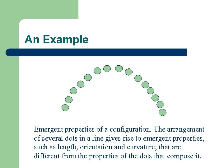An Example Emergent properties of a configuration. The arrangement of several dots in a line gives rise to emergent properties, such as length, orientation and curvature, that are different from the properties of the dots that compose it.

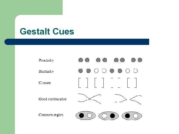Gestalt Cues

And the moral of the story is. . l l l Image segmentation based on low level cues cannot and should not aim to produce a complete final “correct” segmentation. Instead use low-level attributes like color, brightness to sequentially come up with hierarchical partitions. Mid and high-level knowledge can be used to either confirm or select some partition for further attention.

A graph theoretic approach l l A weighted undirected graph G = (V, E) Nodes are points in the feature space Fully connected graph Edge weight w(i, j) is a function of the similarity between nodes i and j. Task: Partition the set V into disjoint sets V 1, . . , Vn, s. t. similarity among nodes in Vi is high and similarity across Vi and Vj is low.

Issues l l What is a good partition ? How can you compute such a partition efficiently ?

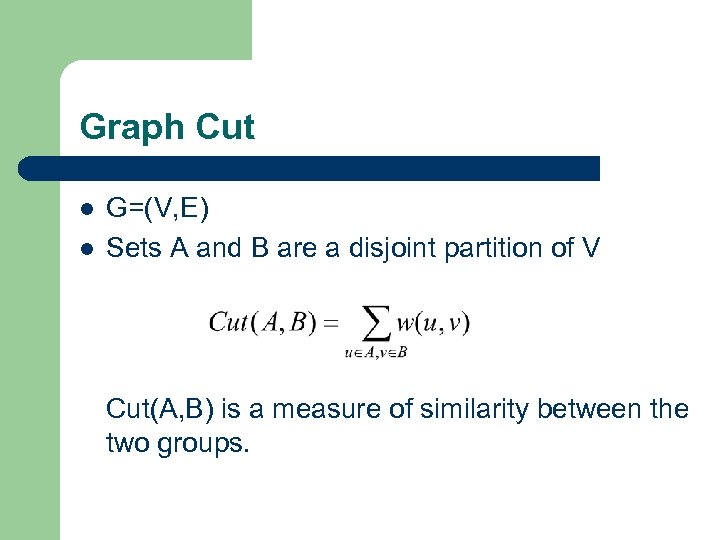Graph Cut l l G=(V, E) Sets A and B are a disjoint partition of V Cut(A, B) is a measure of similarity between the two groups.

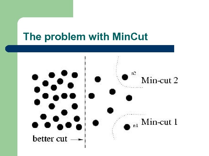
The temptation Cut is a measure of association Minimizing it will give a partition with the maximum disassociation. Efficient poly-time algorithms exist to solve the Min. Cut problem. So why not use it ?

The problem with Min. Cut

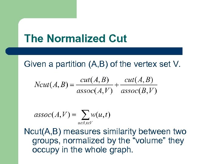The Normalized Cut Given a partition (A, B) of the vertex set V. Ncut(A, B) measures similarity between two groups, normalized by the “volume” they occupy in the whole graph.

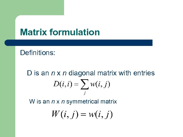Matrix formulation Definitions: D is an n x n diagonal matrix with entries W is an n x n symmetrical matrix

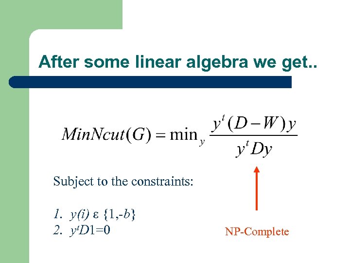After some linear algebra we get. . Subject to the constraints: 1. y(i) ε {1, -b} 2. yt. D 1=0 NP-Complete

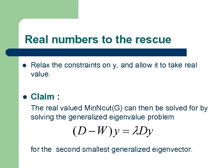Real numbers to the rescue l Relax the constraints on y, and allow it to take real value. l Claim : The real valued Min. Ncut(G) can then be solved for by solving the generalized eigenvalue problem for the second smallest generalized eigenvector.

Proof l Rewrite the equation as Here Lemma 1: is an eigenvector of the above eigensystem with eigenvalue 0.

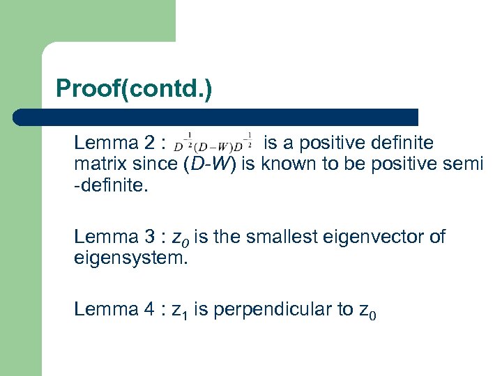Proof(contd. ) Lemma 2 : is a positive definite matrix since (D-W) is known to be positive semi -definite. Lemma 3 : z 0 is the smallest eigenvector of eigensystem. Lemma 4 : z 1 is perpendicular to z 0

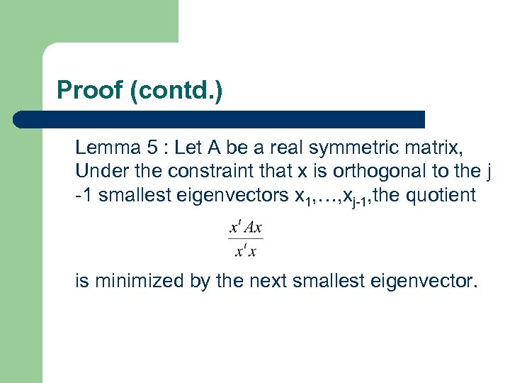Proof (contd. ) Lemma 5 : Let A be a real symmetric matrix, Under the constraint that x is orthogonal to the j -1 smallest eigenvectors x 1, …, xj-1, the quotient is minimized by the next smallest eigenvector.

Finally. . 1. 2. 3. 4. By lemma 1 we have y 0=1 is an eigenvector of the eigensystem with eigenvalue 0. It is the “smallest” eigenvector. Hence by lemma 2, the second smallest eigenvector (y 1) will minimize the Ncut equation. By lemma 3 and 4 z 1 tz 0= y 1 t. D 1=0

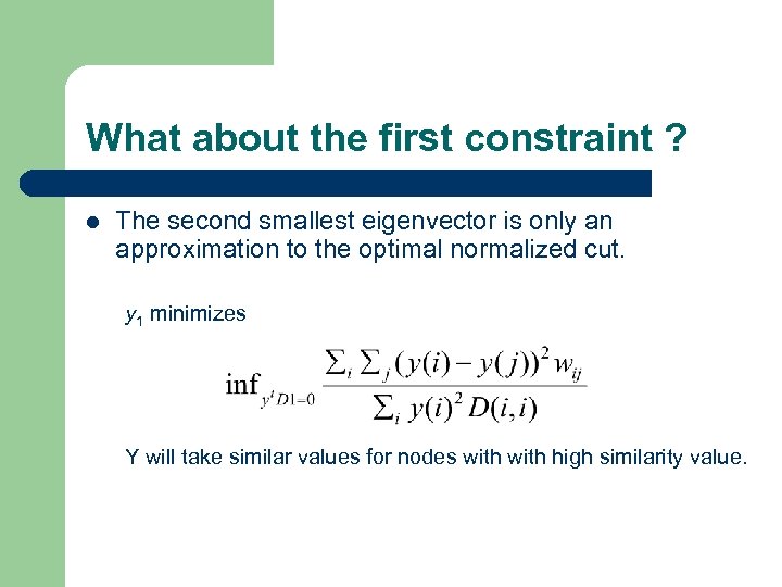What about the first constraint ? l The second smallest eigenvector is only an approximation to the optimal normalized cut. y 1 minimizes Y will take similar values for nodes with high similarity value.

The grouping algorithm 1. 2. 3. Given an image, set up the weighted graph G=(E, V). Set the weight on the edges connecting two nodes as a measure of the similarity between the nodes. Solve (D-W)x=λDx for eigenvectors with the smallest eigenvalues. Use the second smallest eigenvector to bipartition the graph.

Details. . l The eigenvector takes continuous values, how do use it to segment the image ? 1. 2. 3. 4. Choose 0 as the splitting point. Find the median of the eigenvector and use that as the splitting point Search amongst l evenly spaced points for one which gives the best exact Ncut value. Impose a stability criterion on the eigenvector.

Stability ? l l l Since we allow the eigenvectors to take real values. Some eigenvectors might take a smooth continuous form. We want vectors that have sharp discontinuities, indicating separation between regions. Measure the smoothness of the vector, and stop partitioning when the smoothness value falls below a threshold.

Detail. . (Contd. ) l How do you partition images with multiple segments ? 1. The higher order eigenvectors contain information about subpartitions. Keep splitting till Ncut exceeds some pre-specified value. Problem : Numerical Error 2. Recursively run the algorithm on successive subgraphs. Problem : Computationally Expensive and the stability criterion might prevent correct partitioning.

Simultanous P-way cut 1. 2. 3. Use the first n eigenvectors as ndimensional indicator vectors of each point. This is equivalent to imbedding each point in an n-dimensional space. Perform k-means clustering in this new space to create p’>p clusters. Use the original 2 -way Ncut or a greedy strategy to merge these p’ partitions into p partitions.

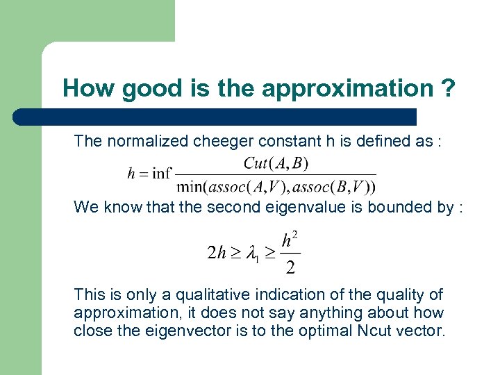How good is the approximation ? The normalized cheeger constant h is defined as : We know that the second eigenvalue is bounded by : This is only a qualitative indication of the quality of approximation, it does not say anything about how close the eigenvector is to the optimal Ncut vector.

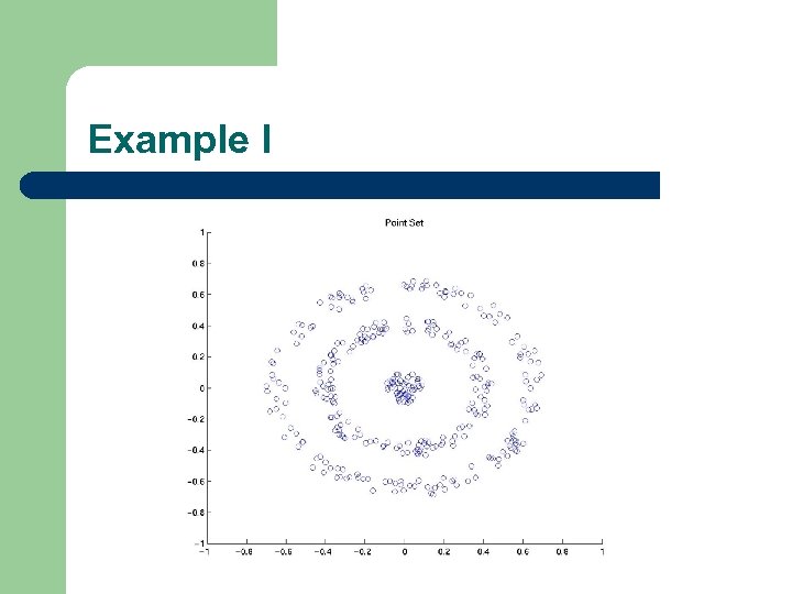Example I

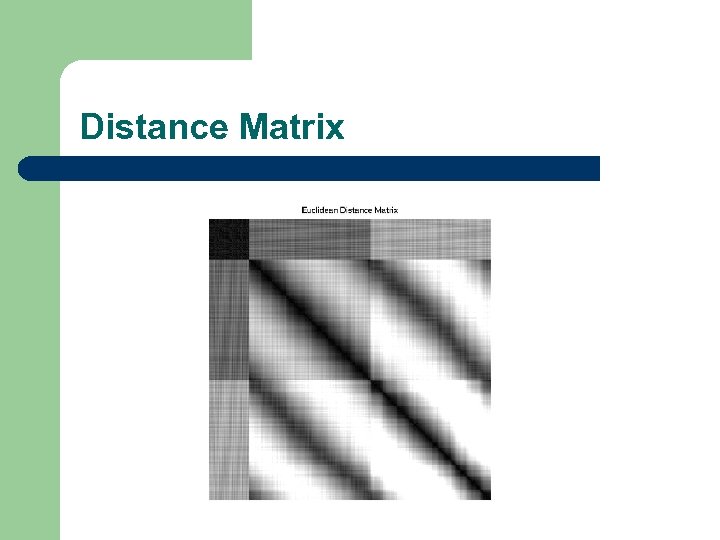Distance Matrix

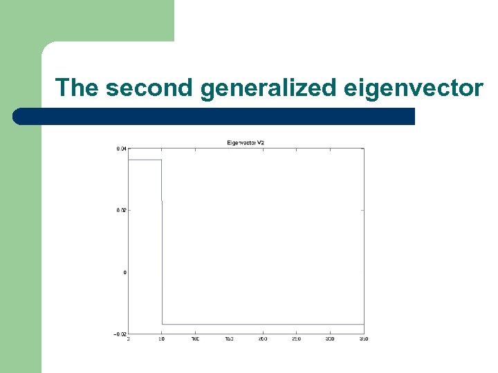The second generalized eigenvector

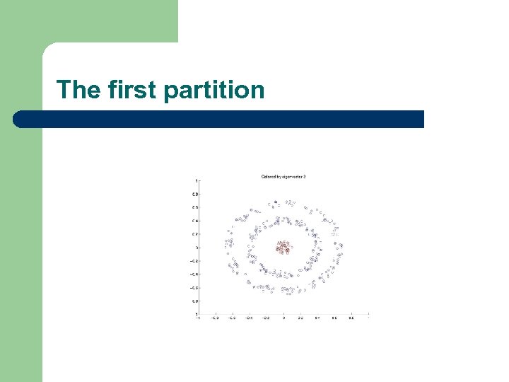The first partition

The second generalized eigenvector

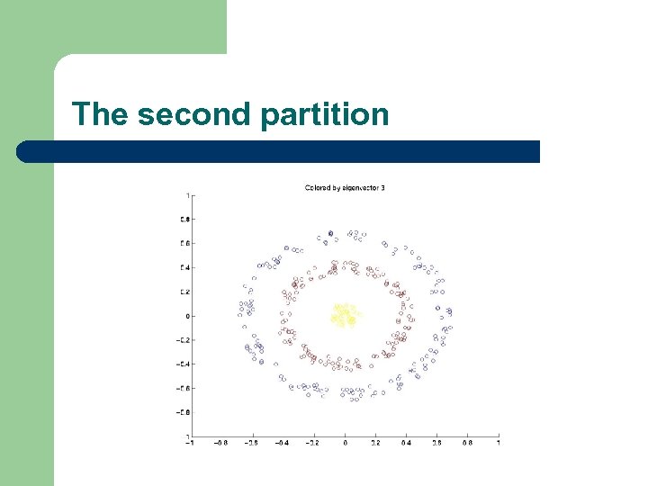The second partition

The fourth generalized eigenvector

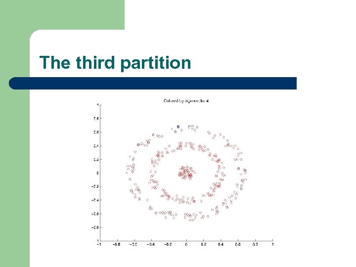The third partition

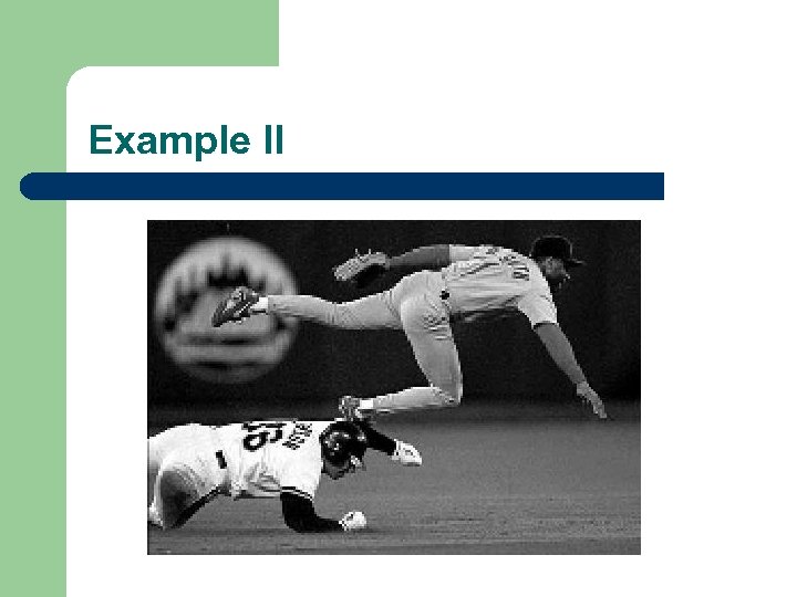Example II

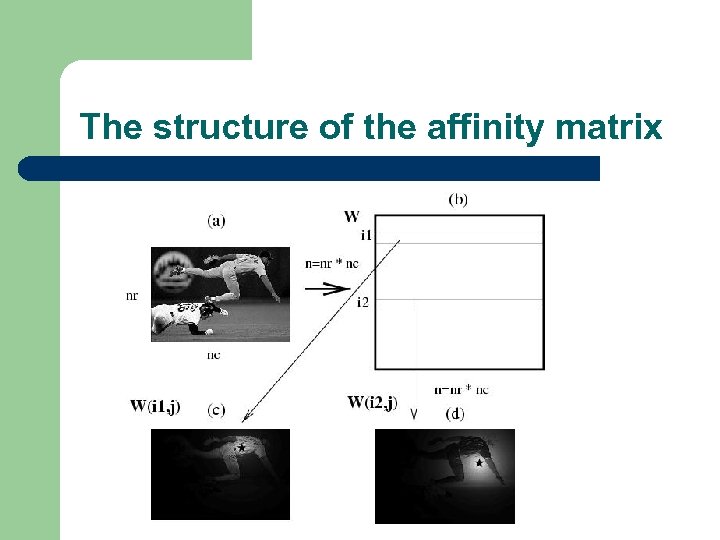The structure of the affinity matrix

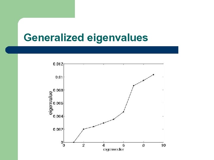Generalized eigenvalues

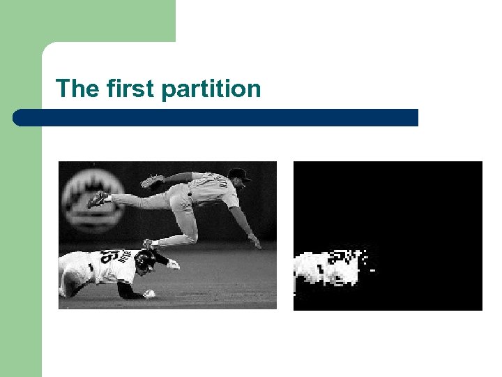The first partition

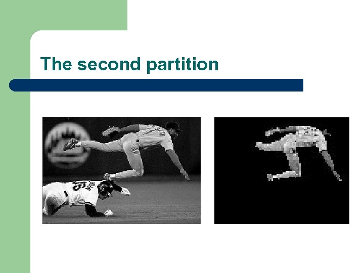The second partition

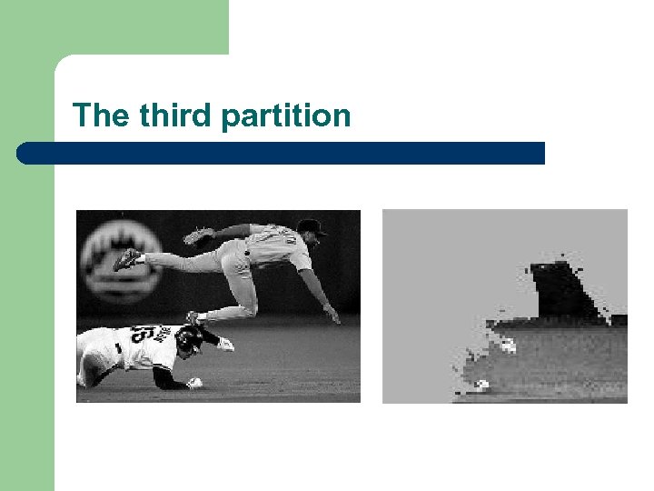The third partition

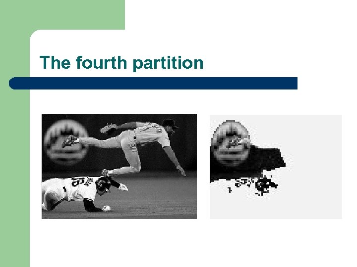The fourth partition

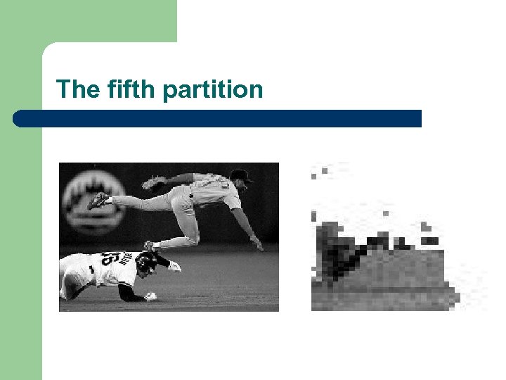The fifth partition

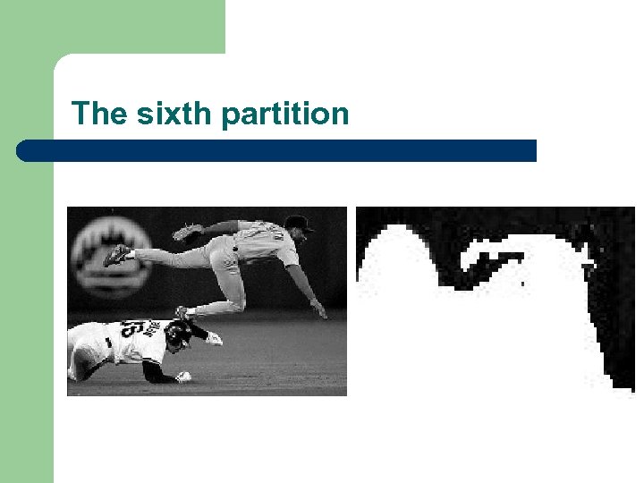The sixth partition

Complexity Issues l l Finding Eigenvectors for an n x n matrix is O(n 3) operation. This is extremely expensive One solution is to make the affinity matrix sparse. Only consider nearby points. Efficient methods exist for finding eigenvectors of sparse matrices. Even with the best methods, its not possible to perform this task in real time.

The Nystrom method l l Belongie et. al. made the observation that the affinity matrix has very low rank i. e. the matrix has very few unique rows. Hence its possible to approximate the eigenvectors of the whole affinity matrix by linearly interpolating the eigenvectors of a small randomly sampled sub-matrix. This method is fast enough to give real-time performance. This is also referred to as the Nystrom method in operator theory.

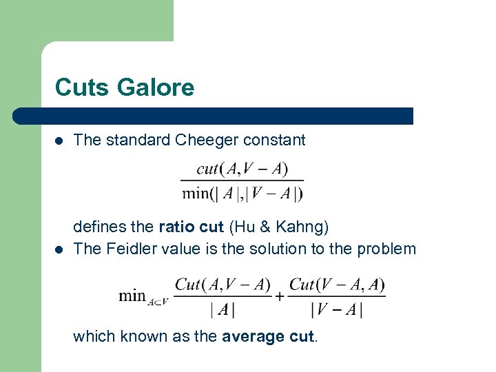Cuts Galore l The standard Cheeger constant l defines the ratio cut (Hu & Kahng) The Feidler value is the solution to the problem which known as the average cut.

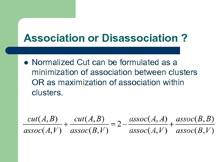Association or Disassociation ? l Normalized Cut can be formulated as a minimization of association between clusters OR as maximization of association within clusters.

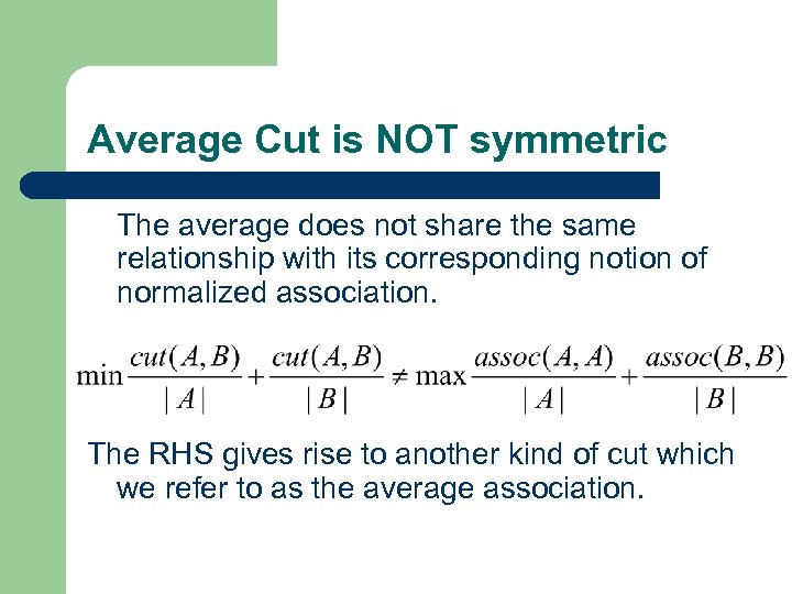Average Cut is NOT symmetric The average does not share the same relationship with its corresponding notion of normalized association. The RHS gives rise to another kind of cut which we refer to as the average association.

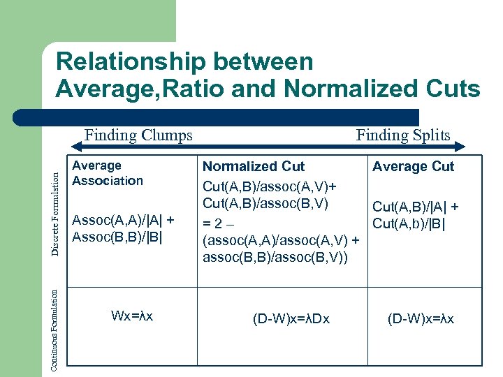Relationship between Average, Ratio and Normalized Cuts Continuous Formulation Discrete Formulation Finding Clumps Average Association Assoc(A, A)/|A| + Assoc(B, B)/|B| Wx=λx Finding Splits Normalized Cut Average Cut(A, B)/assoc(A, V)+ Cut(A, B)/assoc(B, V) Cut(A, B)/|A| + =2– Cut(A, b)/|B| (assoc(A, A)/assoc(A, V) + assoc(B, B)/assoc(B, V)) (D-W)x=λDx (D-W)x=λx

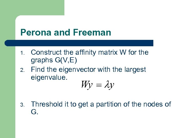Perona and Freeman 1. 2. 3. Construct the affinity matrix W for the graphs G(V, E) Find the eigenvector with the largest eigenvalue. Threshold it to get a partition of the nodes of G.

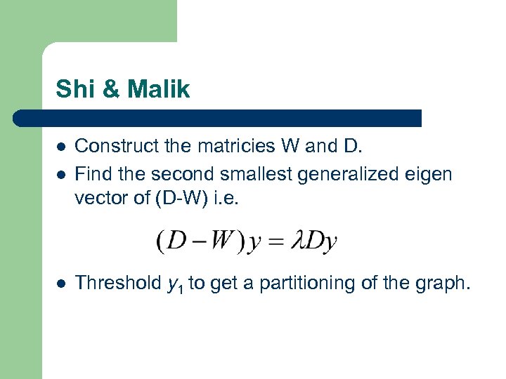Shi & Malik l Construct the matricies W and D. Find the second smallest generalized eigen vector of (D-W) i. e. l Threshold y 1 to get a partitioning of the graph. l

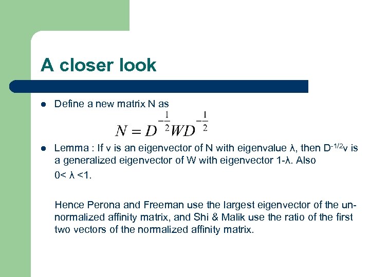A closer look l Define a new matrix N as l Lemma : If v is an eigenvector of N with eigenvalue λ, then D-1/2 v is a generalized eigenvector of W with eigenvector 1 -λ. Also 0< λ <1. Hence Perona and Freeman use the largest eigenvector of the unnormalized affinity matrix, and Shi & Malik use the ratio of the first two vectors of the normalized affinity matrix.

Scott and Longuet-Higgins l l Construct the matrix V whose columns are the k eigenvectors of W Normalize the rows of V Construct the matrix Q = V VT Segment points using Q. If i and j belong to the same cluster, Q(i, j)=1, 0 if they belong to different groups.

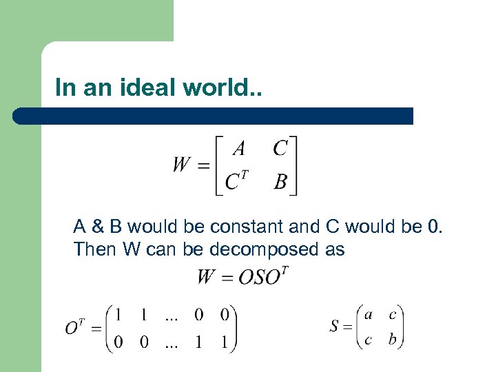In an ideal world. . A & B would be constant and C would be 0. Then W can be decomposed as

And that tells us. . 1. If V is a 2 x 2 matrix whose columns are the first two eigen vectors of W. Then V = ODR, where D is a 2 x 2 diagonal matrix and R is a 2 x 2 rotation matrix. Now if W(i, j) on depends on the membership of i and j : 1. 2. 3. If v 1 is the indicator vector(first eigenvector of W) of the PF algorithm, then if i and j belong to the same cluster then v(i) = v(j). If v 1 is the indicator vector(second generalized eigenvector of W) and if i and j belong to the same cluster then v(i) = v(j). If Q is the indicator matrix in the SLH method, then Q(i, j)=1, 0 otherwise.

Non-constant Matricies Let A, B be arbitrary positive matrices and C=0. l l l Let v be the PF indicator vector. If λ(A)1 > λ(B)1 , then v(i) >0 for all points belonging to the first cluster and v(j) =0 for points belonging to the second cluster. Let v be the SM indicator vector, then v(i)=v(j) if points i and j belong to the same cluster. If λ(B)1 > |λ(A)2 | and λ(A)1 > |λ(B)2 | then Q(i, j) = 1 if i, j belong to the same cluster, 0 otherwise.

Conclusions l l Normalized cut presents a new optimality criterion for partitioning a graph into clusters. Ncut is normalized measure of disassociation and minimizing it is equivalent to maximizing association. The discrete problem corresponding to Min Ncut is NPComplete. We solve an approximate version of the Min. Ncut problem by converting it into a generalized eigenvector problem.

Conclusions (contd. ) l l There a number of approaches which use the eigenvectors of matrices related to the affinity matrix of a graph. Three of these methods can be shown to be based on the top eigenvectors of the affinity matrix. They differ in two ways 1. Which eigenvectors to look at. 2. Whether to normalize the matrix or not ?

References 1. 2. Normalized Cut and Image Segmentation – Jianbo Shi and Jitendra Malik Segmentation using eigenvectors: a unifying view – Yair Weiss

Acknowledgements l l l Serge Belongie for sharing hours of excitement and details of Linear Algebra and associated wonders. Ben Leong for sharing his figures. And the music of Tool for keeping me company.