IMAGE RESTORATION Outline A model of

IMAGE RESTORATION

Outline • A model of the image degradation / restoration process • Noise models • Restoration in the presence of noise only – spatial filtering • Periodic noise reduction by frequency domain filtering • Linear, position-invariant degradations • Estimating the degradation function • Inverse filtering & Wiener filtering • Constrained Least square filtering • Geometric mean filter • Geometric and spatial transformation

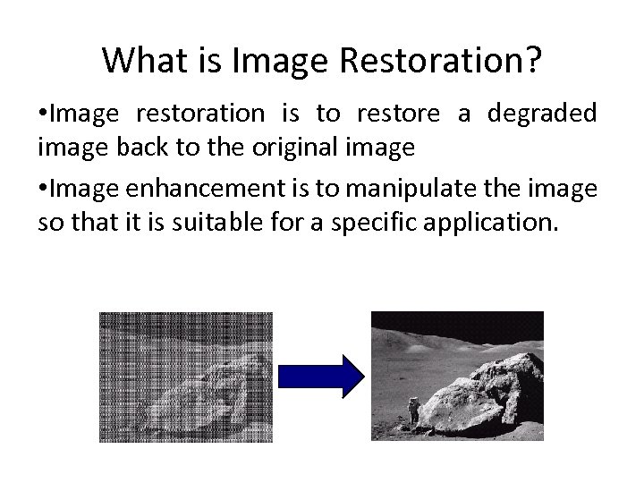What is Image Restoration? • Image restoration is to restore a degraded image back to the original image • Image enhancement is to manipulate the image so that it is suitable for a specific application.

Image Restoration Image restoration attempts to restore images that have been degraded – Identify the degradation process and attempt to reverse it – Similar to image enhancement, but more objective 4

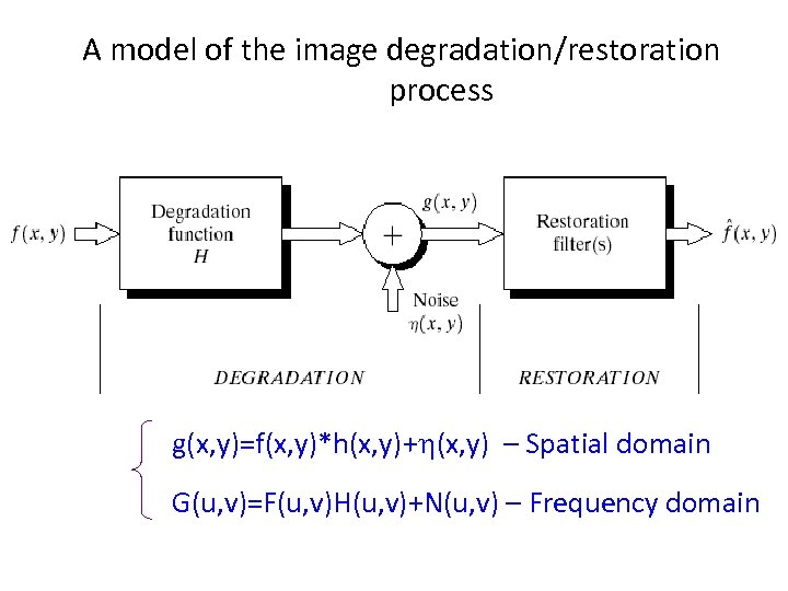A model of the image degradation/restoration process g(x, y)=f(x, y)*h(x, y)+h(x, y) – Spatial domain G(u, v)=F(u, v)H(u, v)+N(u, v) – Frequency domain

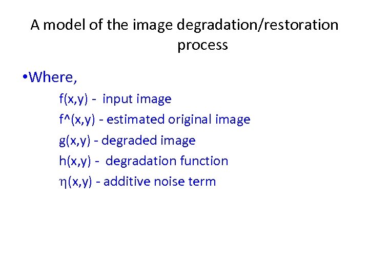A model of the image degradation/restoration process • Where, f(x, y) - input image f^(x, y) - estimated original image g(x, y) - degraded image h(x, y) - degradation function h(x, y) - additive noise term

Noise models • Sources of noise – Image acquisition (digitization) - Imaging sensors can be affected by ambient conditions – Image transmission - Interference can be added to an image during transmission • Spatial properties of noise – Statistical behavior of the gray-level values of pixels – Noise parameters, correlation with the image • Frequency properties of noise – Fourier spectrum – Ex. white noise (a constant Fourier spectrum)

Noise models • Noise model is decided based on understanding of the physics of the sources of noise. –Gaussian: poor illumination –Rayleigh: range image –Gamma(Erlang), Exponential: laser imaging –Impulse: faulty switch during imaging –Uniform: least used

Noise probability density functions • Noise cannot be predicted but can be approximately described in statistical way using the probability density function (PDF)

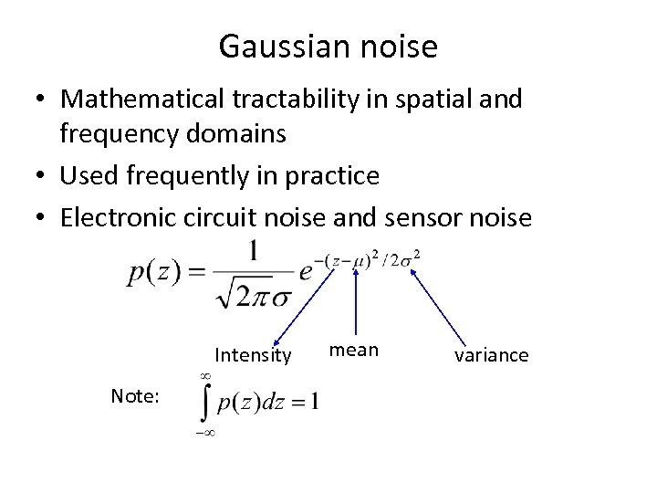Gaussian noise • Mathematical tractability in spatial and frequency domains • Used frequently in practice • Electronic circuit noise and sensor noise Intensity Note: mean variance

Gaussian noise PDF 70% in [(m-s), (m+s)] 95% in [(m-2 s), (m+2 s)]

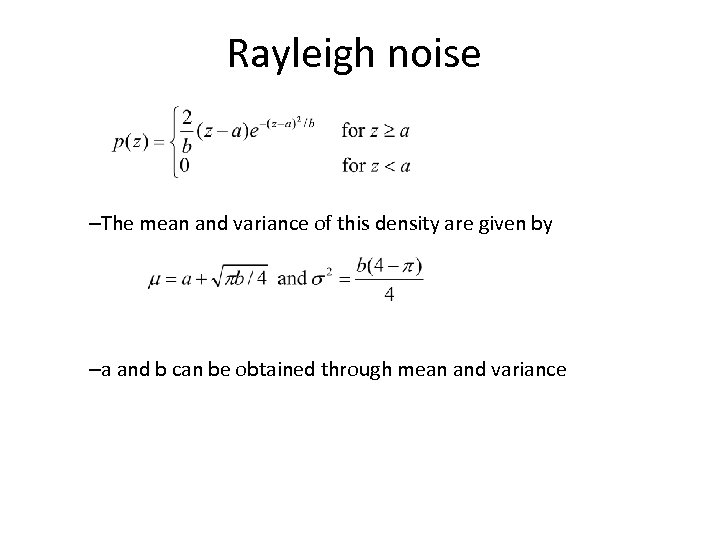Rayleigh noise –The mean and variance of this density are given by –a and b can be obtained through mean and variance

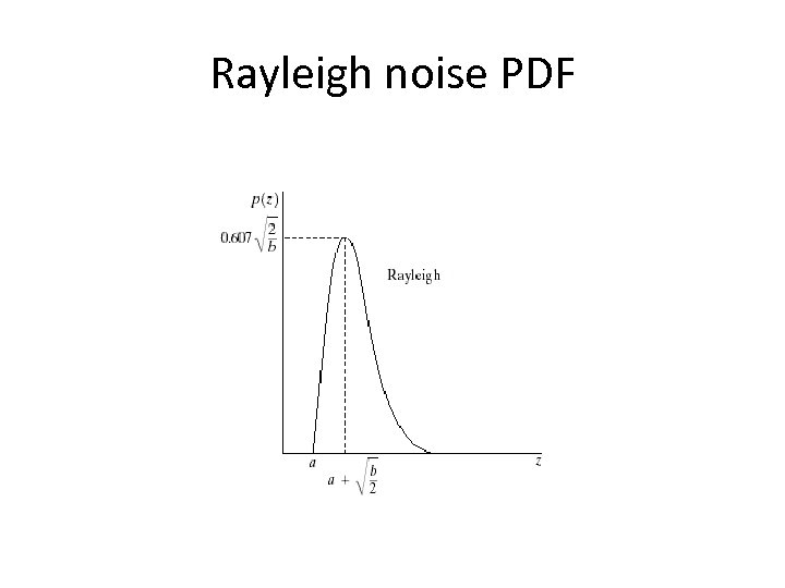Rayleigh noise PDF

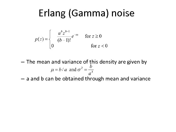Erlang (Gamma) noise – The mean and variance of this density are given by – a and b can be obtained through mean and variance

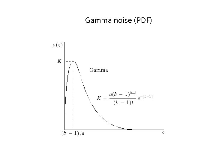Gamma noise (PDF)

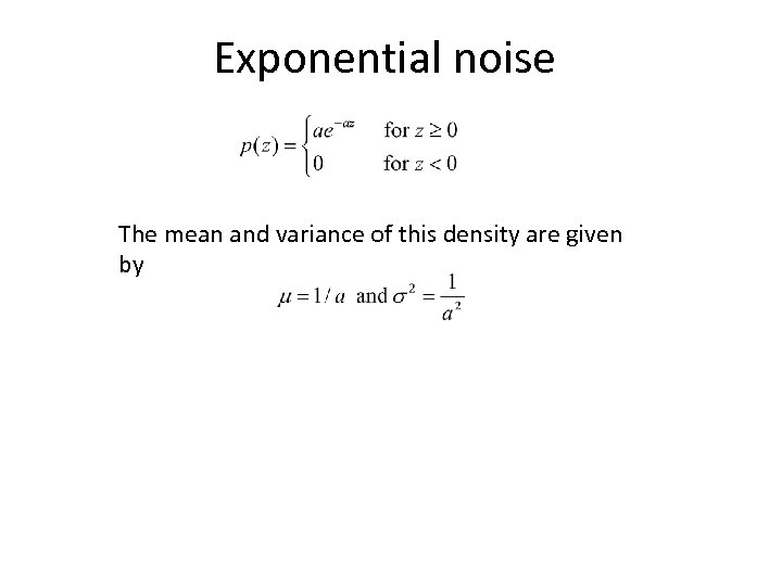Exponential noise The mean and variance of this density are given by

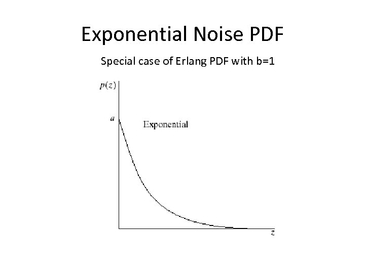Exponential Noise PDF Special case of Erlang PDF with b=1

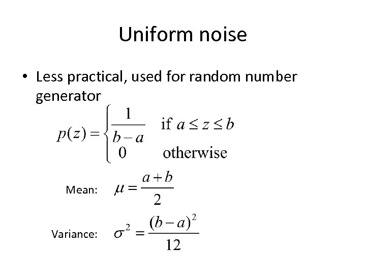Uniform noise • Less practical, used for random number generator Mean: Variance:

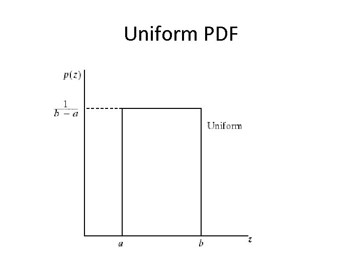Uniform PDF z

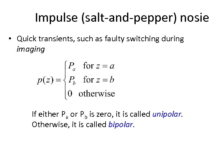Impulse (salt-and-pepper) nosie • Quick transients, such as faulty switching during imaging If either Pa or Pb is zero, it is called unipolar. Otherwise, it is called bipolar.

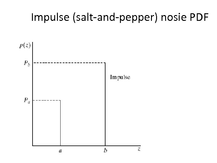Impulse (salt-and-pepper) nosie PDF

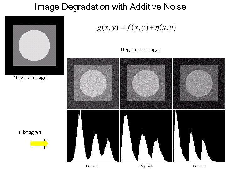Image Degradation with Additive Noise Degraded images Original image Histogram

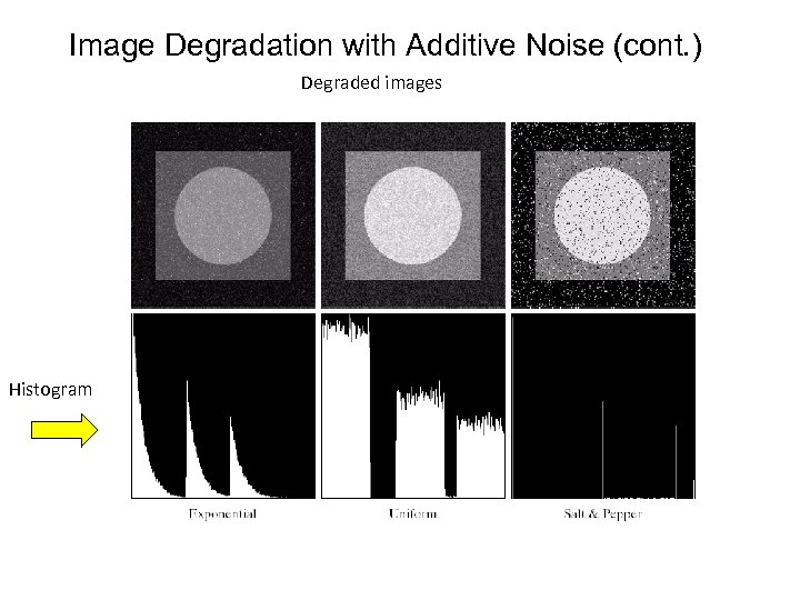Image Degradation with Additive Noise (cont. ) Degraded images Histogram

Periodic noise • Is an image that arises from electrical and electromechanical interference during image acquisition • It can be observed by visual inspection both in the spatial domain and frequency domain • can be reduced significantly via frequency domain filtering

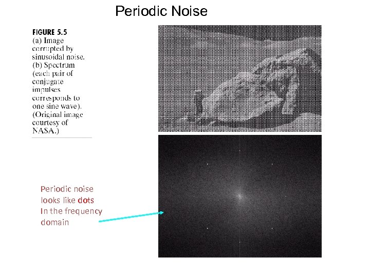Periodic Noise Periodic noise looks like dots In the frequency domain

Estimation of noise parameters • Periodic noise – Observe the frequency spectrum • Random noise with unknown PDFs – Case 1: imaging system is available • Capture images of “flat” environment – Case 2: noisy images available • Take a strip from constant area • Draw the histogram and observe it • Measure the mean and variance

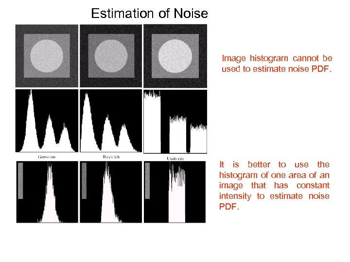Estimation of Noise Image histogram cannot be used to estimate noise PDF. It is better to use the histogram of one area of an image that has constant intensity to estimate noise PDF.

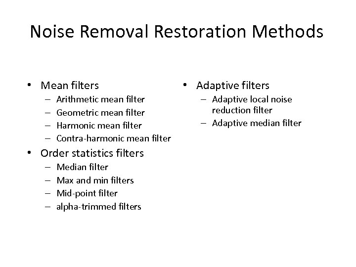Noise Removal Restoration Methods • Mean filters – – Arithmetic mean filter Geometric mean filter Harmonic mean filter Contra-harmonic mean filter • Order statistics filters – – Median filter Max and min filters Mid-point filter alpha-trimmed filters • Adaptive filters – Adaptive local noise reduction filter – Adaptive median filter

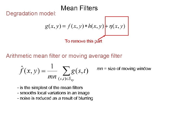Degradation model: Mean Filters To remove this part Arithmetic mean filter or moving average filter mn = size of moving window - is the simplest of the mean filters - smooths local variations in an image - noise is reduced as a result of blurring

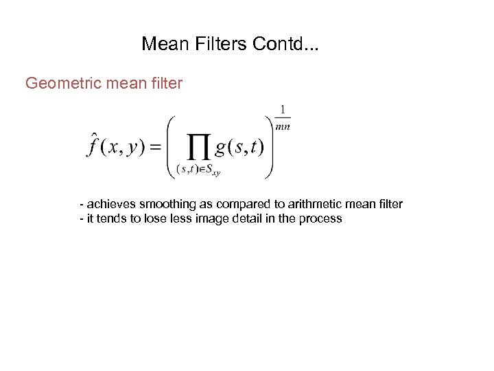Mean Filters Contd. . . Geometric mean filter - achieves smoothing as compared to arithmetic mean filter - it tends to lose less image detail in the process

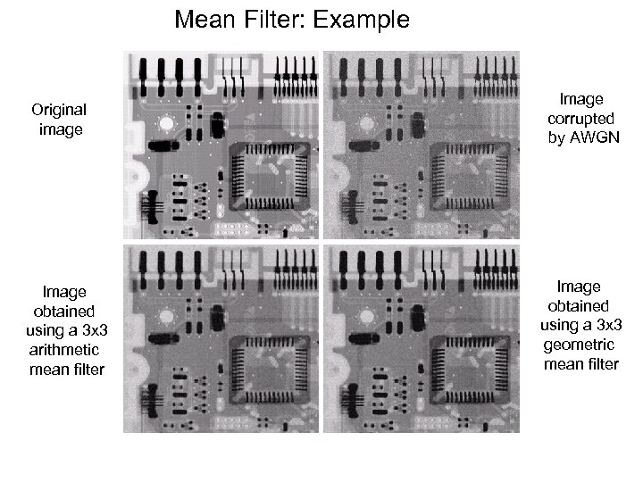Mean Filter: Example Original image Image obtained using a 3 x 3 arithmetic mean filter Image corrupted by AWGN Image obtained using a 3 x 3 geometric mean filter

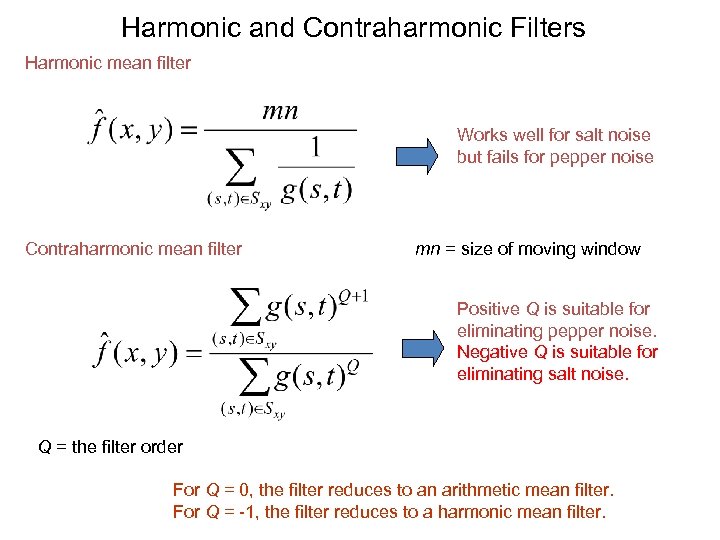Harmonic and Contraharmonic Filters Harmonic mean filter Works well for salt noise but fails for pepper noise Contraharmonic mean filter mn = size of moving window Positive Q is suitable for eliminating pepper noise. Negative Q is suitable for eliminating salt noise. Q = the filter order For Q = 0, the filter reduces to an arithmetic mean filter. For Q = -1, the filter reduces to a harmonic mean filter.

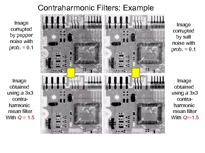Contraharmonic Filters: Example Image corrupted by pepper noise with prob. = 0. 1 Image corrupted by salt noise with prob. = 0. 1 Image obtained using a 3 x 3 contraharmonic mean filter With Q = 1. 5 Image obtained using a 3 x 3 contraharmonic mean filter With Q=-1. 5

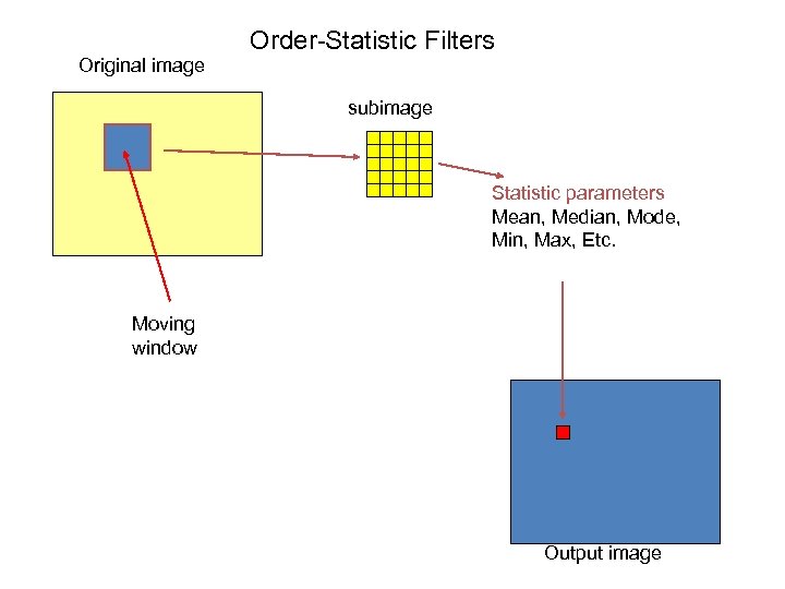Order-Statistic Filters Original image subimage Statistic parameters Mean, Median, Mode, Min, Max, Etc. Moving window Output image

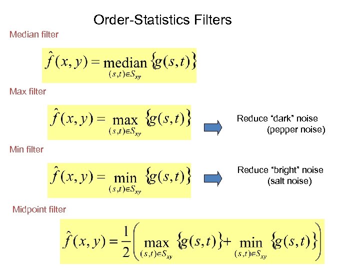Order-Statistics Filters Median filter Max filter Reduce “dark” noise (pepper noise) Min filter Reduce “bright” noise (salt noise) Midpoint filter

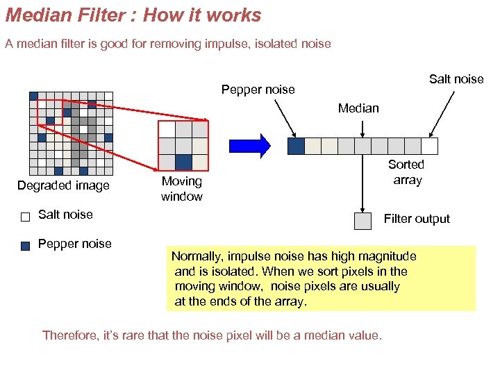Median Filter : How it works A median filter is good for removing impulse, isolated noise Salt noise Pepper noise Median Degraded image Moving window Salt noise Pepper noise Sorted array Filter output Normally, impulse noise has high magnitude and is isolated. When we sort pixels in the moving window, noise pixels are usually at the ends of the array. Therefore, it’s rare that the noise pixel will be a median value.

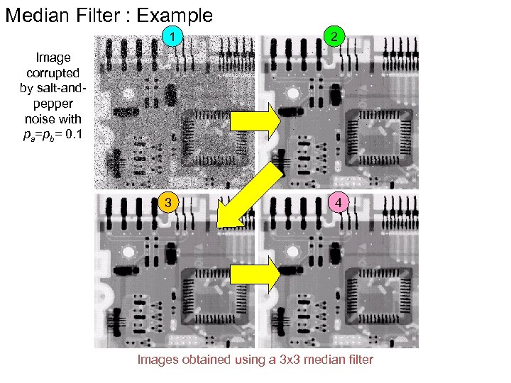Median Filter : Example 1 2 Image corrupted by salt-andpepper noise with pa=pb= 0. 1 3 4 Images obtained using a 3 x 3 median filter

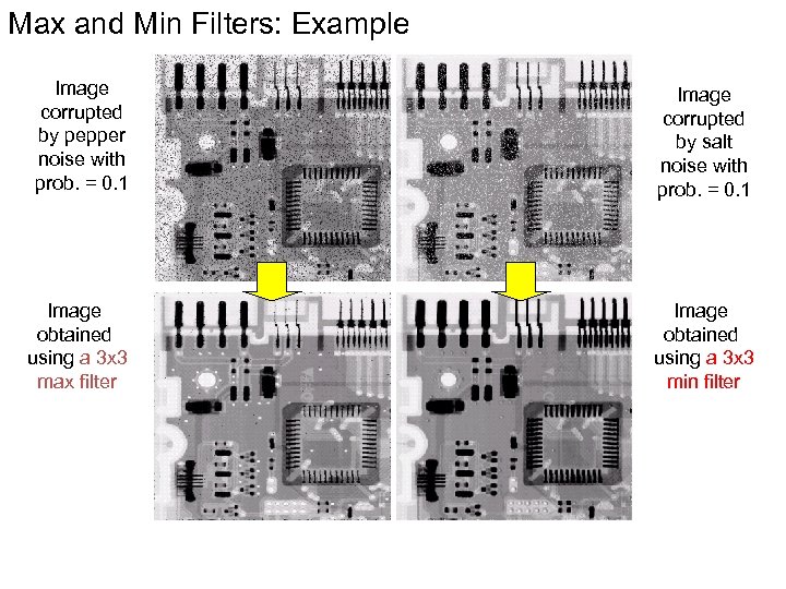Max and Min Filters: Example Image corrupted by pepper noise with prob. = 0. 1 Image corrupted by salt noise with prob. = 0. 1 Image obtained using a 3 x 3 max filter Image obtained using a 3 x 3 min filter

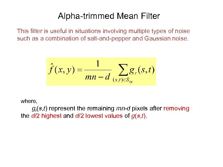Alpha-trimmed Mean Filter This filter is useful in situations involving multiple types of noise such as a combination of salt-and-pepper and Gaussian noise. where, gr(s, t) represent the remaining mn-d pixels after removing the d/2 highest and d/2 lowest values of g(s, t).

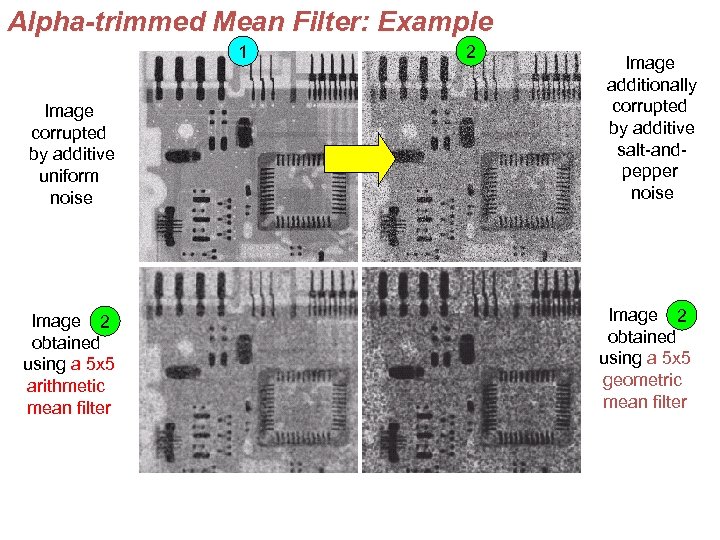Alpha-trimmed Mean Filter: Example 1 Image corrupted by additive uniform noise Image 2 obtained using a 5 x 5 arithmetic mean filter 2 Image additionally corrupted by additive salt-andpepper noise Image 2 obtained using a 5 x 5 geometric mean filter

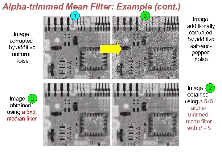Alpha-trimmed Mean Filter: Example (cont. ) 1 Image corrupted by additive uniform noise Image 2 obtained using a 5 x 5 median filter 2 Image additionally corrupted by additive salt-andpepper noise Image 2 obtained using a 5 x 5 alphatrimmed mean filter with d = 5

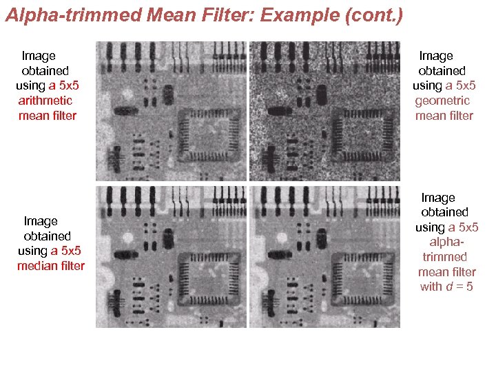Alpha-trimmed Mean Filter: Example (cont. ) Image obtained using a 5 x 5 arithmetic mean filter Image obtained using a 5 x 5 geometric mean filter Image obtained using a 5 x 5 median filter Image obtained using a 5 x 5 alphatrimmed mean filter with d = 5

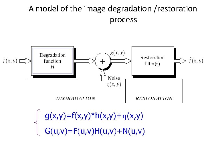A model of the image degradation /restoration process g(x, y)=f(x, y)*h(x, y)+h(x, y) G(u, v)=F(u, v)H(u, v)+N(u, v)

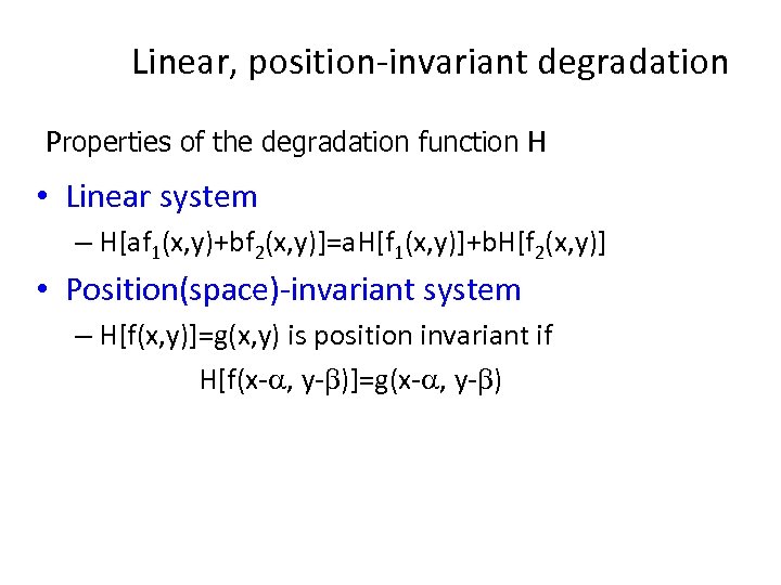Linear, position-invariant degradation Properties of the degradation function H • Linear system – H[af 1(x, y)+bf 2(x, y)]=a. H[f 1(x, y)]+b. H[f 2(x, y)] • Position(space)-invariant system – H[f(x, y)]=g(x, y) is position invariant if H[f(x-a, y-b)]=g(x-a, y-b)

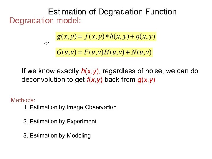Estimation of Degradation Function Degradation model: or If we know exactly h(x, y), regardless of noise, we can do deconvolution to get f(x, y) back from g(x, y). Methods: 1. Estimation by Image Observation 2. Estimation by Experiment 3. Estimation by Modeling

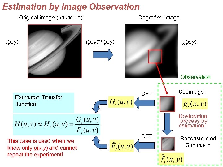Estimation by Image Observation Original image (unknown) f(x, y) Degraded image f(x, y)*h(x, y) g(x, y) Observation Estimated Transfer function DFT Subimage Restoration process by estimation This case is used when we know only g(x, y) and cannot repeat the experiment! DFT Reconstructed Subimage

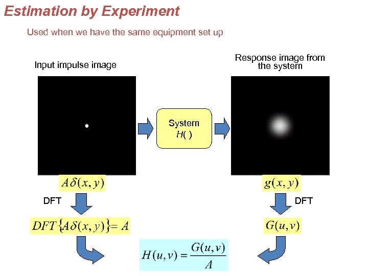Estimation by Experiment Used when we have the same equipment set up Response image from the system Input impulse image System H( ) DFT

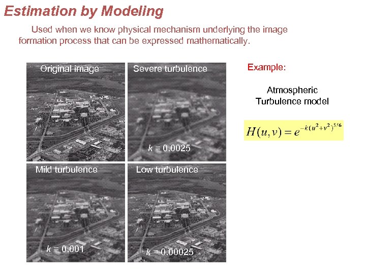Estimation by Modeling Used when we know physical mechanism underlying the image formation process that can be expressed mathematically. Original image Severe turbulence Example: Atmospheric Turbulence model k = 0. 0025 Mild turbulence Low turbulence k = 0. 001 k = 0. 00025

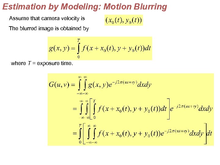Estimation by Modeling: Motion Blurring Assume that camera velocity is The blurred image is obtained by where T = exposure time.

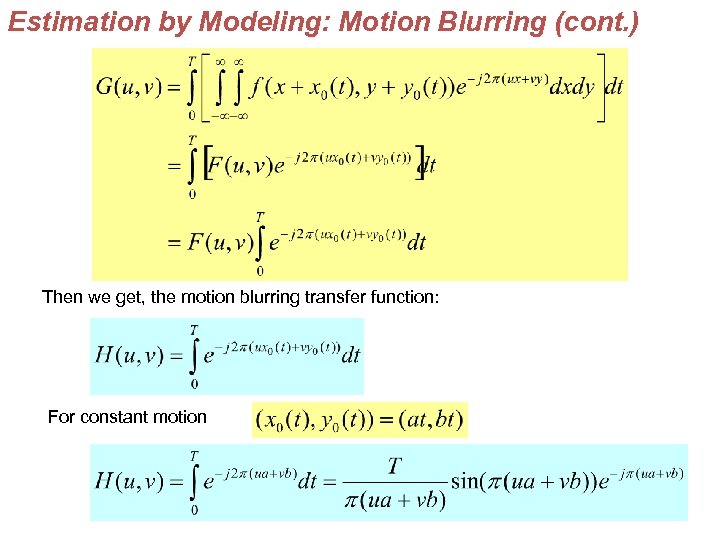Estimation by Modeling: Motion Blurring (cont. ) Then we get, the motion blurring transfer function: For constant motion

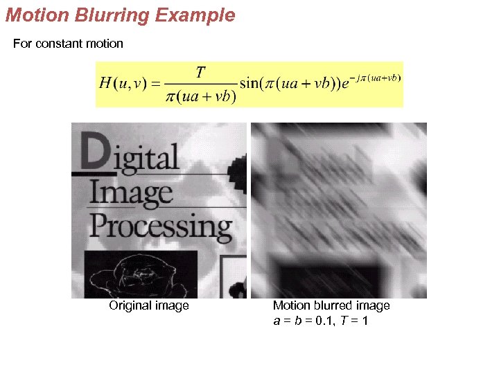Motion Blurring Example For constant motion Original image Motion blurred image a = b = 0. 1, T = 1

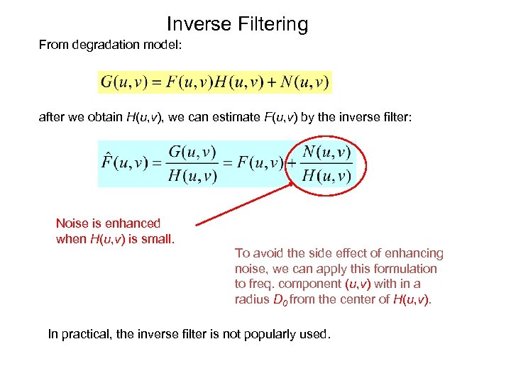Inverse Filtering From degradation model: after we obtain H(u, v), we can estimate F(u, v) by the inverse filter: Noise is enhanced when H(u, v) is small. To avoid the side effect of enhancing noise, we can apply this formulation to freq. component (u, v) with in a radius D 0 from the center of H(u, v). In practical, the inverse filter is not popularly used.

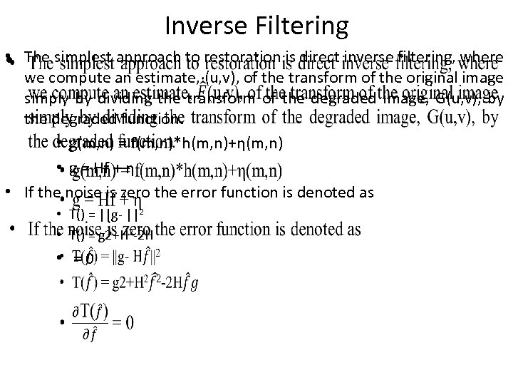Inverse Filtering • The simplest approach to restoration is direct inverse filtering, where • we compute an estimate, (u, v), of the transform of the original image simply by dividing the transform of the degraded image, G(u, v), by the degraded function. • g(m, n) = f(m, n)*h(m, n)+η(m, n) • g = Hf + η • If the noise is zero the error function is denoted as • T() = ||g- ||2 • T() = g 2+H 2 -2 H • = 0

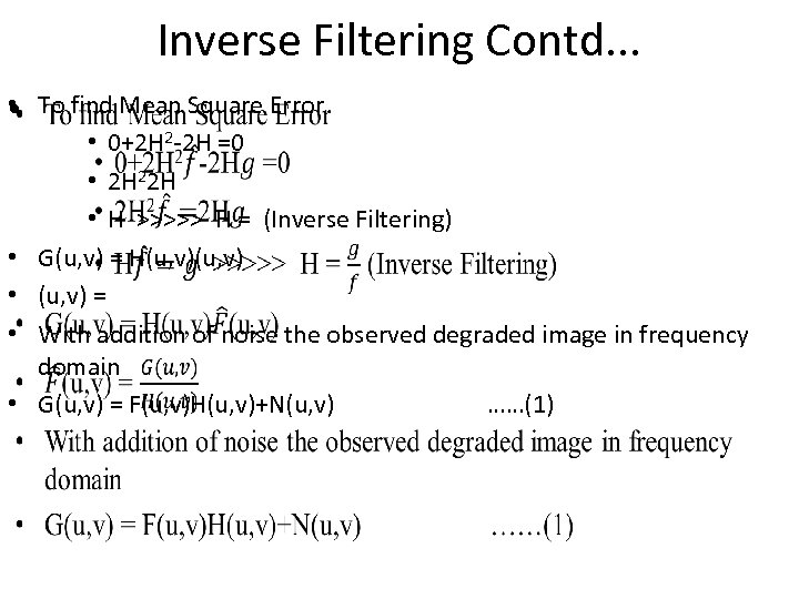Inverse Filtering Contd. . . • To find Mean Square Error • • 0+2 H 2 -2 H =0 • 2 H 22 H • H >>>>> H = (Inverse Filtering) • G(u, v) = H(u, v) • (u, v) = • With addition of noise the observed degraded image in frequency domain • G(u, v) = F(u, v)H(u, v)+N(u, v) ……(1)

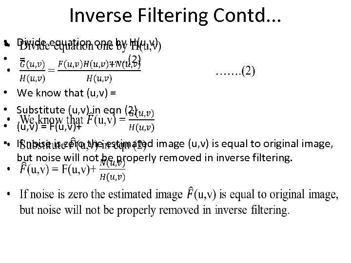Inverse Filtering Contd. . . • Divide equation one by H(u, v) • • = ……. (2) • • We know that (u, v) = Substitute (u, v) in eqn (2) (u, v) = F(u, v)+ If noise is zero the estimated image (u, v) is equal to original image, but noise will not be properly removed in inverse filtering.

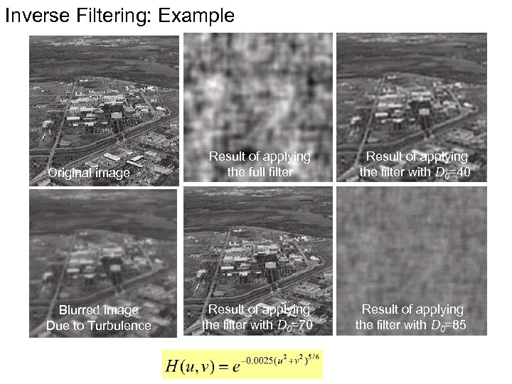Inverse Filtering: Example Original image Blurred image Due to Turbulence Result of applying the full filter Result of applying the filter with D 0=70 Result of applying the filter with D 0=40 Result of applying the filter with D 0=85

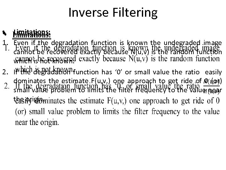Inverse Filtering • Limitations: • 1. Even if the degradation function is known the undegraded image cannot be recovered exactly because N(u, v) is the random function which is not known. 2. If the degradation function has ‘ 0’ or small value the ratio easily dominates the estimate F(u, v, ) one approach to get ride of 0 (or) small value problem to limits the filter frequency to the value near the origin.

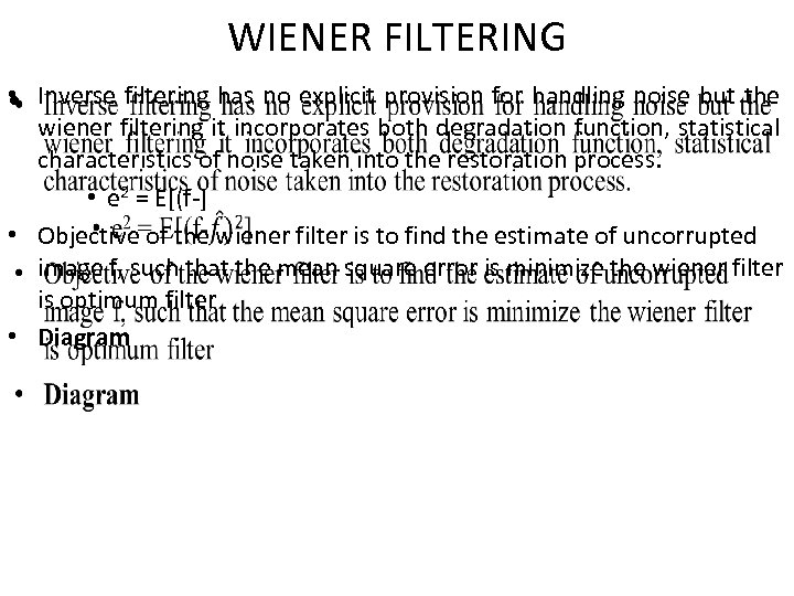WIENER FILTERING • Inverse filtering has no explicit provision for handling noise but the • wiener filtering it incorporates both degradation function, statistical characteristics of noise taken into the restoration process. • e 2 = E[(f-] • Objective of the wiener filter is to find the estimate of uncorrupted image f, such that the mean square error is minimize the wiener filter is optimum filter • Diagram

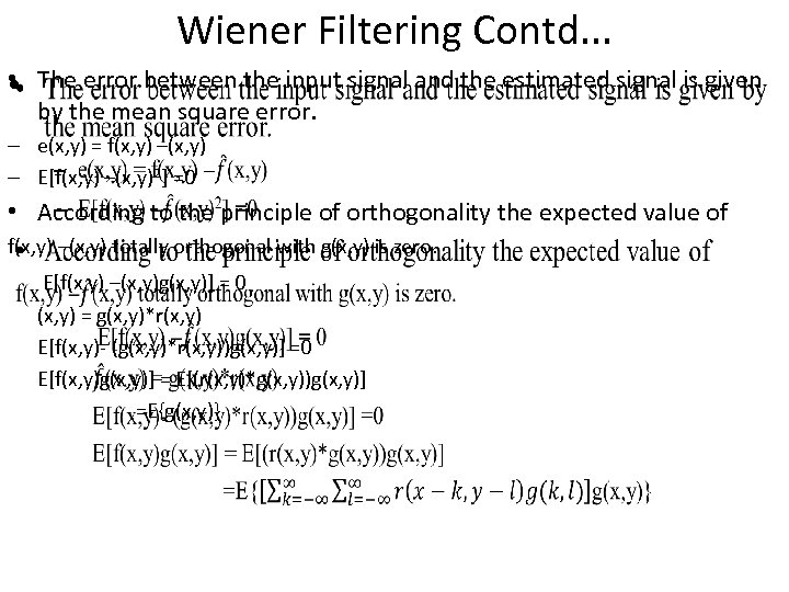Wiener Filtering Contd. . . • The error between the input signal and the estimated signal is given • by the mean square error. – e(x, y) = f(x, y) – E[f(x, y) –(x, y)2] =0 • According to the principle of orthogonality the expected value of f(x, y) –(x, y) totally orthogonal with g(x, y) is zero. E[f(x, y) –(x, y)g(x, y)] = 0 (x, y) = g(x, y)*r(x, y) E[f(x, y)- (g(x, y)*r(x, y))g(x, y)] =0 E[f(x, y)g(x, y)] = E[(r(x, y)*g(x, y))g(x, y)] =E{g(x, y)}

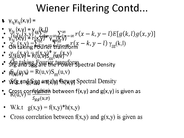Wiener Filtering Contd. . . • • • γfgγfg(x, y) = γfg (x, y) = γgg(k, l) γfg (x, y) = r(x, y)* γgg(x, y) On taking Fourier transform Sfg(u, v) = R(u, v)Sgg(u, v) Sfg and Sgg are the Power Spectral Density R(u, v) = W. k. t g(x, y) = f(x, y)*h(x, y) Cross correlation between f(x, y) and g(x, y) is given as

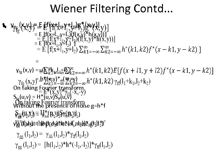Wiener Filtering Contd. . . • γfg (x, y) = E [f(x+l 1, y+l 2)g*(x, y)] • = E [f(x+l 1, y+l 2)(f(x, y)*h(x, y))] = E [f(x+l 1, y+l 2) ] = γfg (x, y) = ff(l 1+k 1, l 2+k 2) = h*(x, y)*ff(-x, -y) On taking Fourier transform Sfg(u, v) = H*(u, v)Sff(u, v) Without the presence of noise g=h*f γgg (l 1, l 2) = γhh (l 1, l 2)*ff(l 1, l 2) γgg (l 1, l 2) = [h(l 1, l 2)*h*(-l 1, -l 2)]*ff(l 1, l 2)

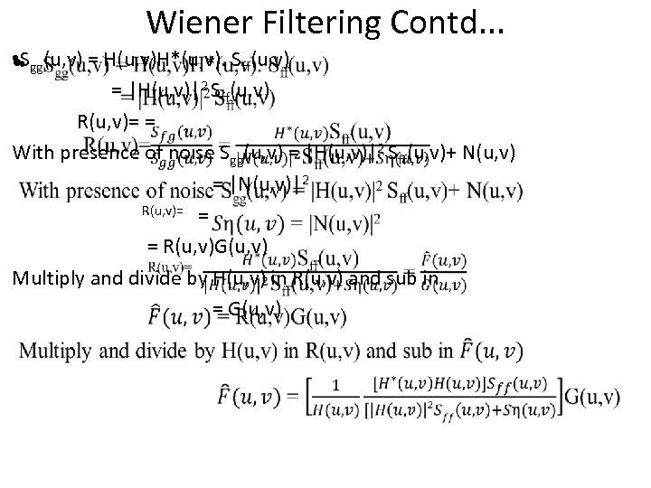Wiener Filtering Contd. . . • Sgg(u, v) = H(u, v)H*(u, v). Sff(u, v) • = |H(u, v)|2 Sff(u, v) R(u, v)= = With presence of noise Sgg(u, v) = |H(u, v)|2 Sff(u, v)+ N(u, v) = |N(u, v)|2 R(u, v)= = = R(u, v)G(u, v) Multiply and divide by H(u, v) in R(u, v) and sub in = G(u, v)

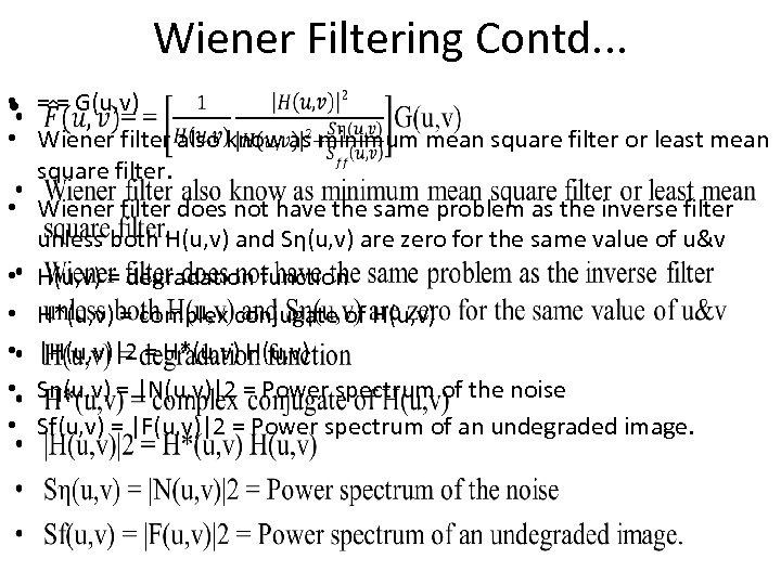Wiener Filtering Contd. . . • = = G(u, v) • • Wiener filter also know as minimum mean square filter or least mean square filter. • Wiener filter does not have the same problem as the inverse filter unless both H(u, v) and Sη(u, v) are zero for the same value of u&v • H(u, v) = degradation function • H*(u, v) = complex conjugate of H(u, v) • |H(u, v)|2 = H*(u, v) H(u, v) • Sη(u, v) = |N(u, v)|2 = Power spectrum of the noise • Sf(u, v) = |F(u, v)|2 = Power spectrum of an undegraded image.

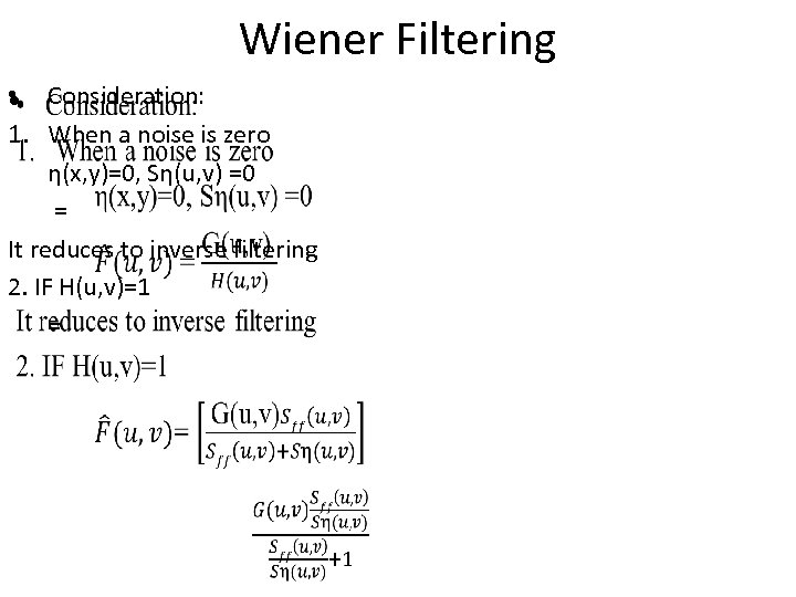Wiener Filtering • Consideration: • 1. When a noise is zero η(x, y)=0, Sη(u, v) =0 = It reduces to inverse filtering 2. IF H(u, v)=1 =

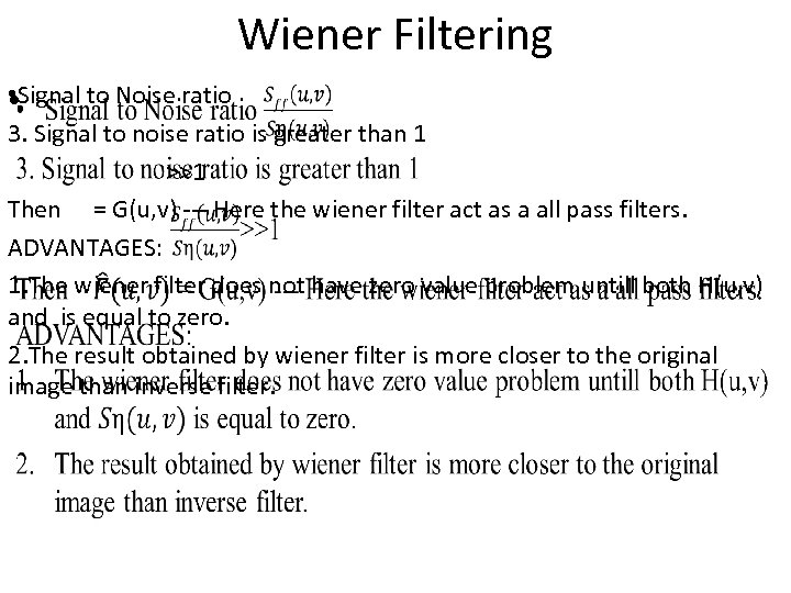Wiener Filtering • Signal to Noise ratio • 3. Signal to noise ratio is greater than 1 >>1 Then = G(u, v) --- Here the wiener filter act as a all pass filters. ADVANTAGES: 1. The wiener filter does not have zero value problem untill both H(u, v) and is equal to zero. 2. The result obtained by wiener filter is more closer to the original image than inverse filter.

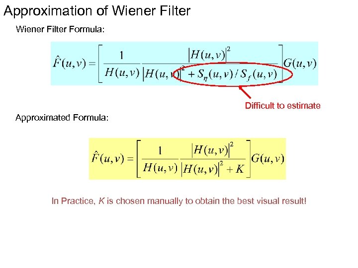Approximation of Wiener Filter Formula: Difficult to estimate Approximated Formula: In Practice, K is chosen manually to obtain the best visual result!

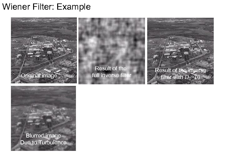Wiener Filter: Example Original image Blurred image Due to Turbulence Result of the full inverse filter Result of the inverse filter with D 0=70 Result of the full Wiener filter

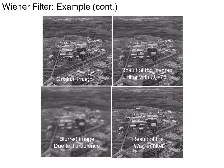Wiener Filter: Example (cont. ) Original image Blurred image Due to Turbulence Result of the inverse filter with D 0=70 Result of the Wiener filter

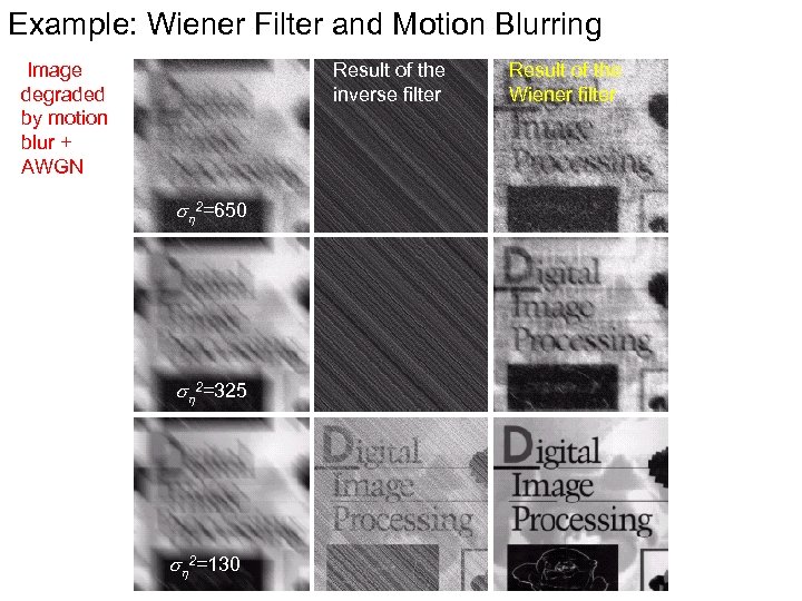Example: Wiener Filter and Motion Blurring Image degraded by motion blur + AWGN Result of the inverse filter sh 2=650 sh 2=325 sh 2=130 Result of the Wiener filter

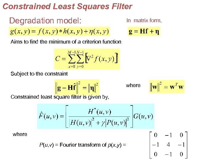Constrained Least Squares Filter Degradation model: In matrix form, Aims to find the minimum of a criterion function Subject to the constraint where Constrained least square filter is given by, where P(u, v) = Fourier transform of p(x, y) =

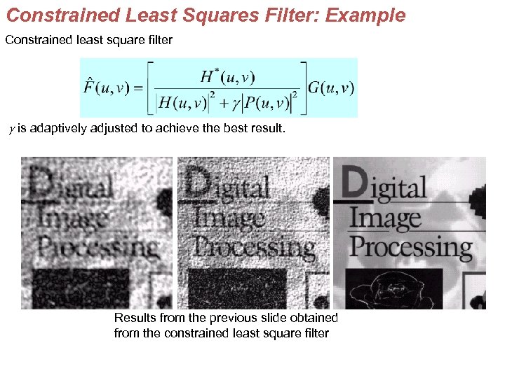Constrained Least Squares Filter: Example Constrained least square filter g is adaptively adjusted to achieve the best result. Results from the previous slide obtained from the constrained least square filter

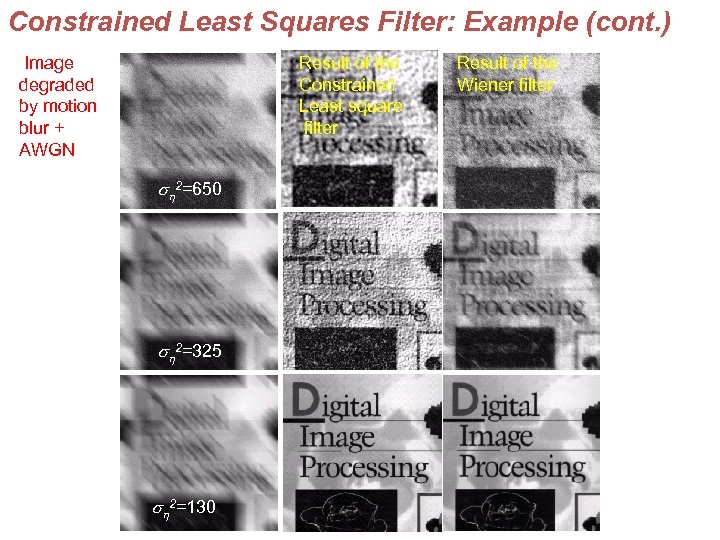Constrained Least Squares Filter: Example (cont. ) Image degraded by motion blur + AWGN Result of the Constrained Least square filter sh 2=650 sh 2=325 sh 2=130 Result of the Wiener filter

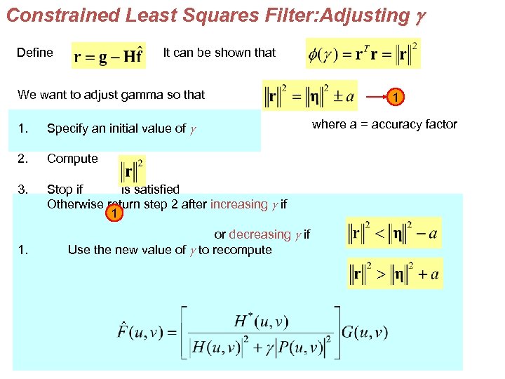Constrained Least Squares Filter: Adjusting g Define It can be shown that We want to adjust gamma so that 1. Specify an initial value of g 2. Compute 3. Stop if is satisfied Otherwise return step 2 after increasing g if 1 1. or decreasing g if Use the new value of g to recompute 1 where a = accuracy factor

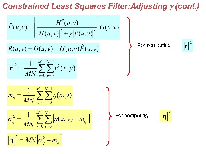Constrained Least Squares Filter: Adjusting g (cont. ) For computing

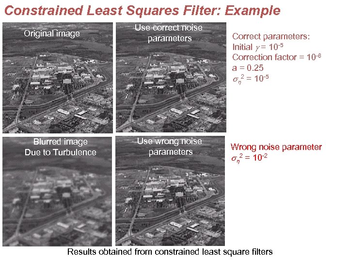Constrained Least Squares Filter: Example Original image Use correct noise parameters Blurred image Due to Turbulence Use wrong noise parameters Correct parameters: Initial g = 10 -5 Correction factor = 10 -6 a = 0. 25 sh 2 = 10 -5 Wrong noise parameter sh 2 = 10 -2 Results obtained from constrained least square filters

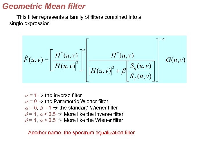Geometric Mean filter This filter represents a family of filters combined into a single expression a = 1 the inverse filter a = 0 the Parametric Wiener filter a = 0, b = 1 the standard Wiener filter b = 1, a < 0. 5 More like the inverse filter b = 1, a > 0. 5 More like the Wiener filter Another name: the spectrum equalization filter

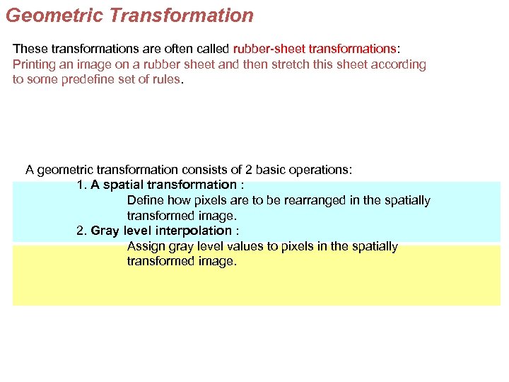Geometric Transformation These transformations are often called rubber-sheet transformations: Printing an image on a rubber sheet and then stretch this sheet according to some predefine set of rules. A geometric transformation consists of 2 basic operations: 1. A spatial transformation : Define how pixels are to be rearranged in the spatially transformed image. 2. Gray level interpolation : Assign gray level values to pixels in the spatially transformed image.

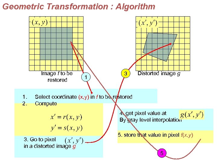Geometric Transformation : Algorithm Image f to be restored 1. 2. 1 3 Distorted image g Select coordinate (x, y) in f to be restored Compute 4. get pixel value at By gray level interpolation 3. Go to pixel in a distorted image g 5. store that value in pixel f(x, y) 5

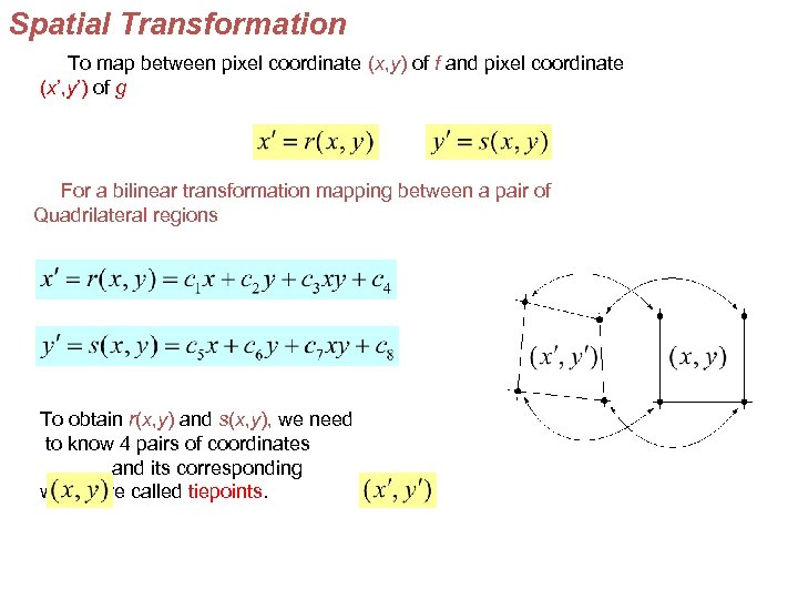Spatial Transformation To map between pixel coordinate (x, y) of f and pixel coordinate (x’, y’) of g For a bilinear transformation mapping between a pair of Quadrilateral regions To obtain r(x, y) and s(x, y), we need to know 4 pairs of coordinates and its corresponding which are called tiepoints.

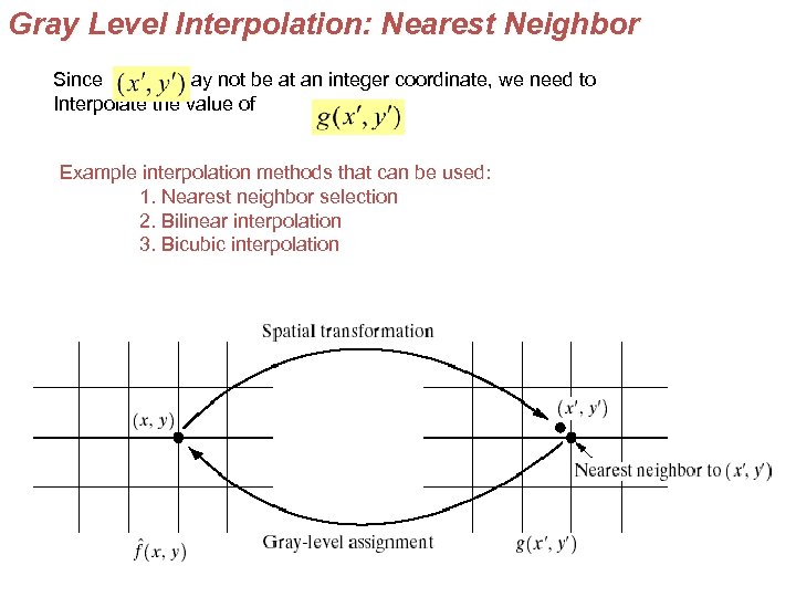Gray Level Interpolation: Nearest Neighbor Since may not be at an integer coordinate, we need to Interpolate the value of Example interpolation methods that can be used: 1. Nearest neighbor selection 2. Bilinear interpolation 3. Bicubic interpolation

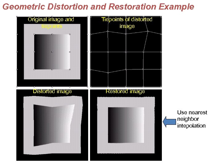Geometric Distortion and Restoration Example Original image and tiepoints Distorted image Tiepoints of distorted image Restored image Use nearest neighbor intepolation

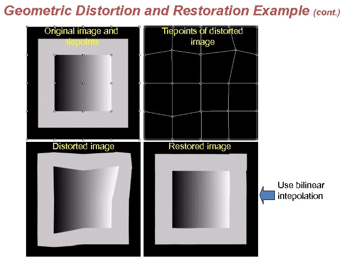Geometric Distortion and Restoration Example (cont. ) Original image and tiepoints Distorted image Tiepoints of distorted image Restored image Use bilinear intepolation

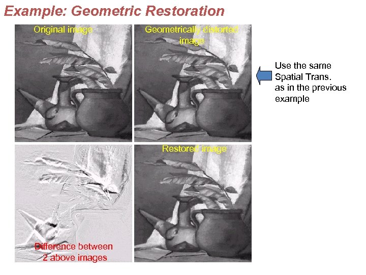Example: Geometric Restoration Original image Geometrically distorted image Use the same Spatial Trans. as in the previous example Restored image Difference between 2 above images