

af00053d170a9289025c3a028f7d6dc8.ppt
- Количество слайдов: 25
 IE 3265 Production & Operations Management Slide Series 2
 Topics for discussion • Product Mix and Product Lifecycle – as they affect the Capacity Planning Problem • The Make or Buy Decision – Its more than $ and ¢! – Break Even Analysis, how we filter in costs • Capacity Planning – When, where and How Much
 Product Issues related to capacity planning • Typical Product Lifecycle help many companies make planning decisions • Facility can be designed for Product Families and the organization tries to match lifecycle demands to keep capacitiy utilized
 The Product Life-Cycle Curve
 The Product/Process Matrix
 Typically Demand Different Production Capacity Design • Is product Typically “One-Off”") Product Mix (Families) Typically Demand Different Production Capacity Design • Is product Typically “One-Off” – These systems have little standardization and require high marketing investment per product – Typically ‘whatever can be made in house’ will be made ‘in house’ – Most designs are highly private and guarded as competitive advantages • Multiple Products in Low Volume – Standard components are made in volume or purchased – Shops use a mixture of flow and fixed site manufacturing layouts
Product Mix (Families) Typically Demand Different Production Capacity Design • Is product Typically “One-Off” – These systems have little standardization and require high marketing investment per product – Typically ‘whatever can be made in house’ will be made ‘in house’ – Most designs are highly private and guarded as competitive advantages • Multiple Products in Low Volume – Standard components are made in volume or purchased – Shops use a mixture of flow and fixed site manufacturing layouts
 Typically Demand Different Production Capacity Design • Few Major (discrete) Products") Product Mix (Families) Typically Demand Different Production Capacity Design • Few Major (discrete) Products in Higher Volume – Purchase most components (its worth standardizing nearly all components) – Make what is highly specialized or provides a competitive advantage – Make decisions are highly dependent of capacity issues • High Volume & Standardized “Commodity” Products – Flow processing all feed products purchased – Manufacturing practices are carefully guarded ‘Trade Secrets’
Product Mix (Families) Typically Demand Different Production Capacity Design • Few Major (discrete) Products in Higher Volume – Purchase most components (its worth standardizing nearly all components) – Make what is highly specialized or provides a competitive advantage – Make decisions are highly dependent of capacity issues • High Volume & Standardized “Commodity” Products – Flow processing all feed products purchased – Manufacturing practices are carefully guarded ‘Trade Secrets’
 Make-Buy Decisions • A difficult problem address by the M-B matrix • Typically requires an analysis of the issues related to People, Processes, and Capacity • Ultimately the problem is addressed economically
 Make – Buy Decision Process Secondary Questions 1. 2. 3. 4. 1. 2. 3. 4. Is the Item Available? Will our Union Allow us to buy? Is outside Quality Acceptable? Are Reliable Sources Available? Is Manufacturing Consistent with our objectives? Do we have Technical Expertise? Is L & MFG capacity available? Must we MFG to utilize existing capacity? Primary Question Can Item be Purchased? Decision NO YES Can Item be Made? YES NO NO = MAKE (if yes continue down) NO = Buy (if yes continue down)
 Make – Buy Decision Process Secondary Questions 1. 2. 3. 4. 1. 2. 3. Primary Question What Alternatives are available to MFG? What is future demand? What are MFG costs? What are Reliability issues that influence purchase or MFG? Is it cheaper to make than buy? What other opportunities are avail. For Capital? What are the future investment implications if item is MFG? What are costs of receiving external Financing? Is Capital Available To Made? Decision NO YES NO NO = Buy (if yes continue down) NO = Buy YES = MAKE
 Break-even Curves for the Make or Buy Problem Cost to Buy = c 1 x Cost to make=K+c 2 x K Break-even quantity
 Example M-B Analysis • Fixed Costs to Purchase consist of: – Vendor Service Costs: • Purchasing Agents Time • Quality/QA Testing Equipment • Overhead/Inventory Set Asides • Fixed Costs to Make (Manufacture) – Machine Overhead • Invested $’s • Machine Depreciation • Maintenance Costs – Order Related Costs (for materials purchase and storage issues)
 Example M-B Analysis • BUY Variable Costs: – Simply the purchase price • Make Variable Costs – Labor/Machine time – Material Consumed – Tooling Costs (consumed)
 Example M-B Analysis • Make or Buy a Machined Component • Purchase: • Fixed Costs for Component: $4000 annually ($20000 over 5 years) • Purchase Price: $38. 00 each • Make Using MFG Process A • Fixed Costs: $145, 750 machine system • Variable cost of labor/overhead is 4 minutes @ $36. 50/hr: $2. 43 • Material Costs: $5. 05/piece • Total Variable costs: $7. 48/each
 Example M-B Analysis • Make on MFG. Process B: • Fixed Cost of Machine System: $312, 500 • Variable Labor/overhead cost is 36 sec @ 45. 00/hr: $0. 45 • Material Costs: $5. 05 • Formula for Breakeven: F a + V a. X = F b + V b. X X is Break even quantity Fi is Fixed cost of Option i Vi is Variable cost of Option i
/(38 -7. 48)}") Example M-B Analysis • Buy vs MFG 1: BE is {(145750 -20000)/(38 -7. 48)} = 4120 units • Buy vs MFG 2: BE is {(312500 -20000)/(38 -5. 5)} = 9000 units • MFG 1 vs MFG 2: BE is {(312500 -145750)/(7. 48 -5. 50)} = 68620 units
Example M-B Analysis • Buy vs MFG 1: BE is {(145750 -20000)/(38 -7. 48)} = 4120 units • Buy vs MFG 2: BE is {(312500 -20000)/(38 -5. 5)} = 9000 units • MFG 1 vs MFG 2: BE is {(312500 -145750)/(7. 48 -5. 50)} = 68620 units
 Capacity Strategy Fundamental issues: – Amount. When adding capacity, what is the optimal amount to add? • Too little means that more capacity will have to be added shortly afterwards. • Too much means that capital will be wasted. – Timing. What is the optimal time between adding new capacity? – Type. Level of flexibility, automation, layout, process, level of customization, outsourcing, etc.
 Three Approaches to Capacity Strategy • Policy A: Try not to run short. Here capacity must lead demand, so on average there will be excess capacity. • Policy B: Build to forecast. Capacity additions should be timed so that the firm has excess capacity half the time and is short half the time. • Policy C: Maximize capacity utilization. Capacity additions lag demand, so that average demand is never met.
 Capacity Leading and Lagging Demand
 Determinants of Capacity Strategy • Highly competitive industries (commodities, large number of suppliers, limited functional difference in products, time sensitive customers) – here shortages are very costly. Use Type A Policy. • Monopolistic environment where manufacturer has power over the industry: Use Type C Policy. (Intel, Lockheed/Martin). • Products that obsolete quickly, such as computer products. Want type C policy, but in competitive industry, such as computers, you will be gone if you cannot meet customer demand. Need best of both worlds: Dell Computer.
 Mathematical Model for Timing of Capacity Additions Let D = Annual Increase in Demand x = Time interval between adding capacity r = annual discount rate (compounded continuously) f(y) = Cost of operating a plant of capacity y Let C(x) be the total discounted cost of all capacity additions over an infinite horizon if new plants are built every x units of time. Then
 is: Where") Mathematical Model (continued • A typical form for the cost function f(y) is: Where k is a constant of proportionality, and a measures the ratio of incremental to average cost of a unit of plant capacity. A typical value is a=0. 6. Note that a<1 implies economies of scale in plant construction, since
Mathematical Model (continued • A typical form for the cost function f(y) is: Where k is a constant of proportionality, and a measures the ratio of incremental to average cost of a unit of plant capacity. A typical value is a=0. 6. Note that a<1 implies economies of scale in plant construction, since
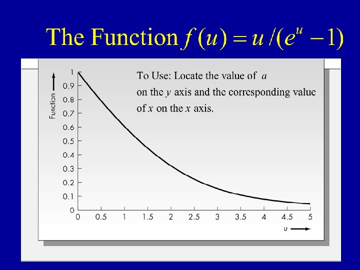
 Hence, It can be shown that this function is minimized at") Mathematical Model (continued) Hence, It can be shown that this function is minimized at x that satisfies the equation: This is known as a transcendental equation, and has no algebraic solution. However, using the graph on the next slide, one can find the optimal value of x or any value of a (0 < a < 1)
Mathematical Model (continued) Hence, It can be shown that this function is minimized at x that satisfies the equation: This is known as a transcendental equation, and has no algebraic solution. However, using the graph on the next slide, one can find the optimal value of x or any value of a (0 < a < 1)
 Issues in Plant Location • • Size of the facility. Product lines. Process technology. Labor requirements. Utilities requirements Environmental issues. International considerations Tax Incentives.