17d787c278d464cee7215813df315d3a.ppt
- Количество слайдов: 37
IBSL Maths: Statistics 1 Discrete random variables This icon indicates the slide contains activities created in Flash. These activities are not editable. For more detailed instructions, see the Getting Started presentation. 1 of 39 © Boardworks Ltd 2005
Discrete random variables Introduction to discrete random variables Contents Cumulative distribution functions Expectation Variance and standard deviation for random variables Discrete uniform distribution Expectation algebra – some key results 2 of 39 © Boardworks Ltd 2005
Discrete random variables The following are all examples of random variables: the number of heads obtained when a coin is tossed four times; the number of prizes I win if I buy 10 tickets in a raffle; the number of cars that pass a checkpoint in a minute; the time (in seconds) it takes to run a 100 m race. In general, a random variable (r. v. ) is a quantity whose value cannot be predicted with certainty before an experiment or enquiry is undertaken. The first three examples above are all discrete random variables – they all take whole number values. 3 of 39 © Boardworks Ltd 2005
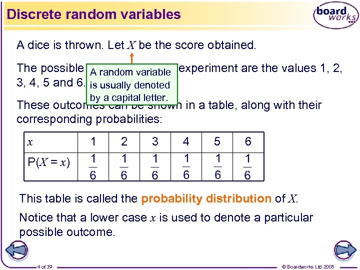
Discrete random variables A dice is thrown. Let X be the score obtained. The possible outcomes of this experiment are the values 1, 2, A random variable 3, 4, 5 and 6. is usually denoted by a capital letter. These outcomes can be shown in a table, along with their corresponding probabilities: 1 x 2 3 4 5 6 P(X = x) This table is called the probability distribution of X. Notice that a lower case x is used to denote a particular possible outcome. 4 of 39 © Boardworks Ltd 2005
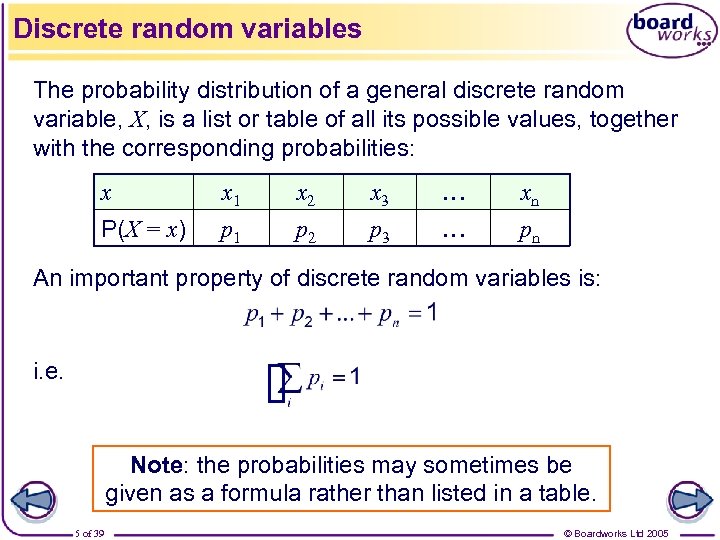
Discrete random variables The probability distribution of a general discrete random variable, X, is a list or table of all its possible values, together with the corresponding probabilities: x x 1 x 2 x 3 … xn P(X = x) p 1 p 2 p 3 … pn An important property of discrete random variables is: i. e. Note: the probabilities may sometimes be given as a formula rather than listed in a table. 5 of 39 © Boardworks Ltd 2005
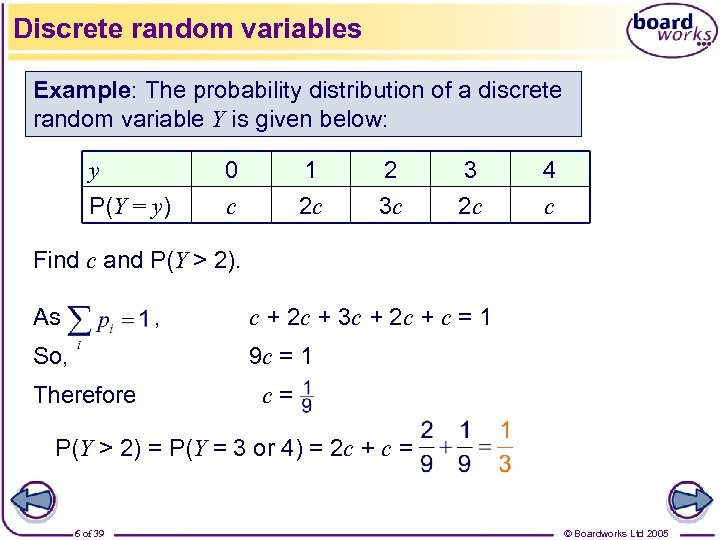
Discrete random variables Example: The probability distribution of a discrete random variable Y is given below: y P(Y = y) 0 c 1 2 c 2 3 c 3 2 c 4 c Find c and P(Y > 2). As , So, c + 2 c + 3 c + 2 c + c = 1 9 c = 1 Therefore c= P(Y > 2) = P(Y = 3 or 4) = 2 c + c = 6 of 39 © Boardworks Ltd 2005
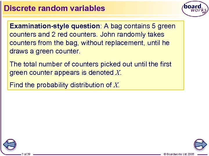
Discrete random variables Examination-style question: A bag contains 5 green counters and 2 red counters. John randomly takes counters from the bag, without replacement, until he draws a green counter. The total number of counters picked out until the first green counter appears is denoted X. Find the probability distribution of X. 7 of 39 © Boardworks Ltd 2005
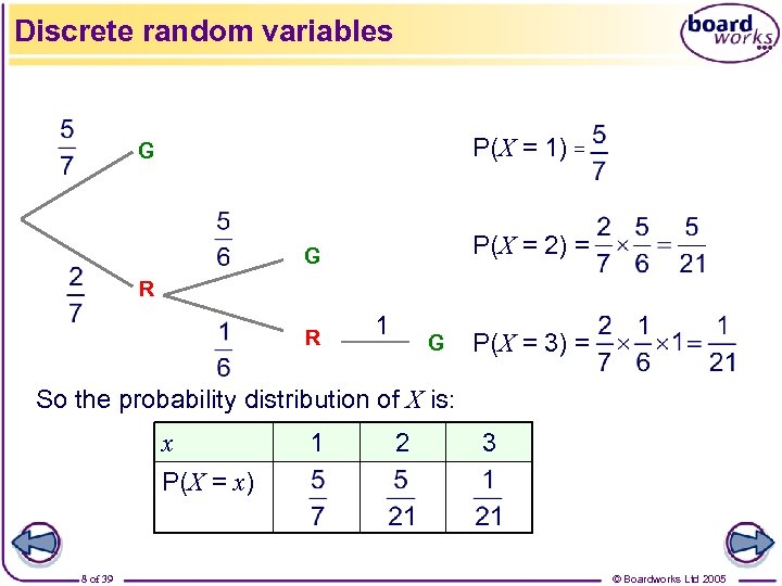
Discrete random variables P(X = 1) = G P(X = 2) = G R R 1 G P(X = 3) = So the probability distribution of X is: x P(X = x) 8 of 39 1 2 3 © Boardworks Ltd 2005
Cumulative distribution functions Introduction to discrete random variables Contents Cumulative distribution functions Expectation Variance and standard deviation for random variables Discrete uniform distribution Expectation algebra – some key results 9 of 39 © Boardworks Ltd 2005
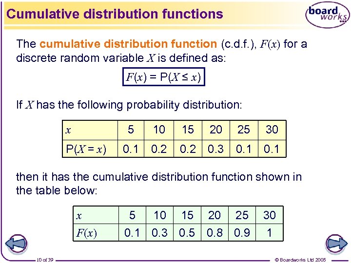
Cumulative distribution functions The cumulative distribution function (c. d. f. ), F(x) for a discrete random variable X is defined as: F(x) = P(X ≤ x) If X has the following probability distribution: 5 x P(X = x) 10 15 20 25 30 0. 1 0. 2 0. 3 0. 1 then it has the cumulative distribution function shown in the table below: x F(x) 10 of 39 5 10 15 20 25 0. 1 0. 3 0. 5 0. 8 0. 9 30 1 © Boardworks Ltd 2005
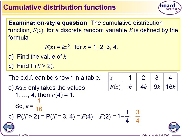
Cumulative distribution functions Examination-style question: The cumulative distribution function, F(x), for a discrete random variable X is defined by the formula F(x) = kx 2 for x = 1, 2, 3, 4. a) Find the value of k. b) Find P(X > 2). The c. d. f. can be shown in a table: a) As x only takes the values 1, …, 4, then F(4) = 1. x F(x) 1 k 2 4 k 3 4 9 k 16 k So, k = b) P(X > 2) = P(X = 3, 4) = F(4) – F(2) = 11 of 39 © Boardworks Ltd 2005
Expectation Introduction to discrete random variables Contents Cumulative distribution functions Expectation Variance and standard deviation for random variables Discrete uniform distribution Expectation algebra – some key results 12 of 39 © Boardworks Ltd 2005
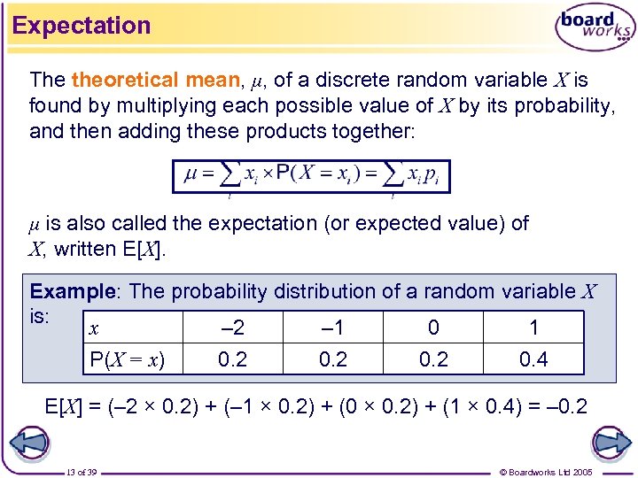
Expectation The theoretical mean, μ, of a discrete random variable X is found by multiplying each possible value of X by its probability, and then adding these products together: μ is also called the expectation (or expected value) of X, written E[X]. Example: The probability distribution of a random variable X is: x – 2 – 1 0 1 P(X = x) 0. 2 0. 4 E[X] = (– 2 × 0. 2) + (– 1 × 0. 2) + (0 × 0. 2) + (1 × 0. 4) = – 0. 2 13 of 39 © Boardworks Ltd 2005
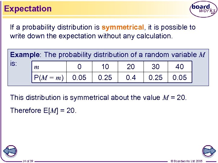
Expectation If a probability distribution is symmetrical, it is possible to write down the expectation without any calculation. Example: The probability distribution of a random variable M is: m 0 10 20 30 40 P(M = m) 0. 05 0. 25 0. 4 0. 25 0. 05 This distribution is symmetrical about the value M = 20. Therefore E[M] = 20. 14 of 39 © Boardworks Ltd 2005
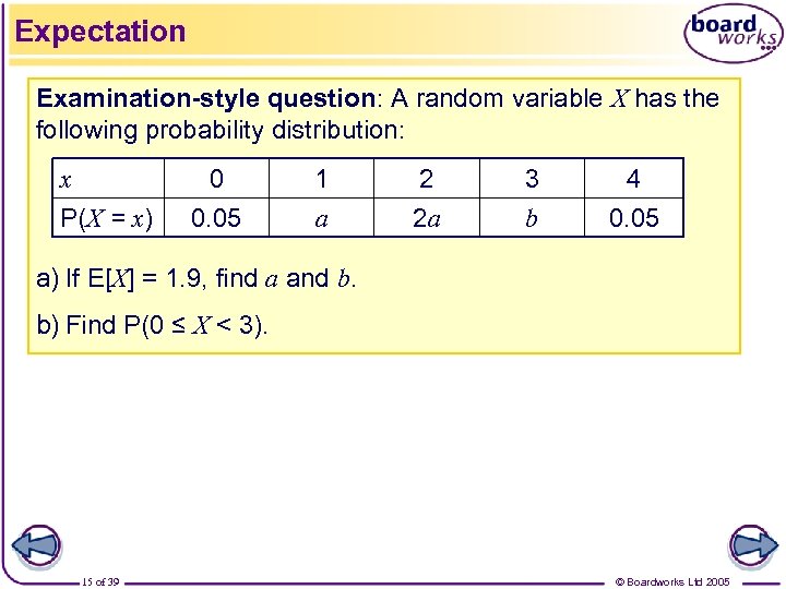
Expectation Examination-style question: A random variable X has the following probability distribution: x P(X = x) 0 0. 05 1 a 2 2 a 3 b 4 0. 05 a) If E[X] = 1. 9, find a and b. b) Find P(0 ≤ X < 3). 15 of 39 © Boardworks Ltd 2005
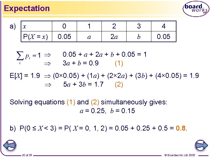
Expectation a) x P(X = x) 0 0. 05 1 a 2 2 a 3 b 4 0. 05 + a + 2 a + b + 0. 05 = 1 3 a + b = 0. 9 (1) E[X] = 1. 9 (0× 0. 05) + (1 a) + (2× 2 a) + (3 b) + (4× 0. 05) = 1. 9 5 a + 3 b = 1. 7 (2) Solving equations (1) and (2) simultaneously gives: a = 0. 25, b = 0. 15 b) P(0 ≤ X < 3) = P( X = 0, 1, 2) = 0. 05 + 0. 25 + 0. 5 = 0. 8. 16 of 39 © Boardworks Ltd 2005
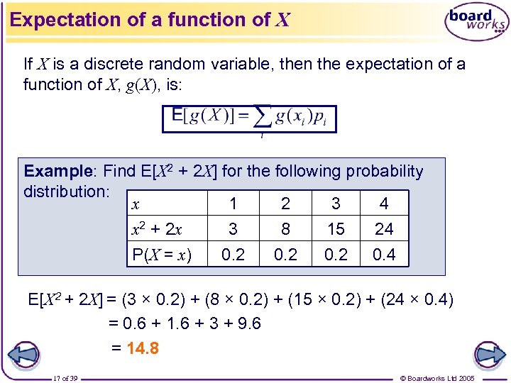
Expectation of a function of X If X is a discrete random variable, then the expectation of a function of X, g(X), is: Example: Find E[X 2 + 2 X] for the following probability distribution: x 1 2 3 4 x 2 + 2 x 3 8 15 24 P(X = x) 0. 2 0. 4 E[X 2 + 2 X] = (3 × 0. 2) + (8 × 0. 2) + (15 × 0. 2) + (24 × 0. 4) = 0. 6 + 1. 6 + 3 + 9. 6 = 14. 8 17 of 39 © Boardworks Ltd 2005
Variance and standard deviation Introduction to discrete random variables Contents Cumulative distribution functions Expectation Variance and standard deviation for random variables Discrete uniform distribution Expectation algebra – some key results 18 of 39 © Boardworks Ltd 2005
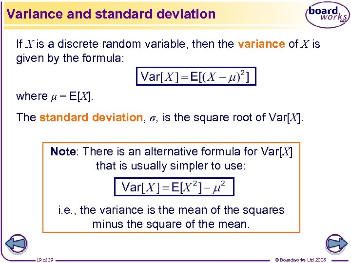
Variance and standard deviation If X is a discrete random variable, then the variance of X is given by the formula: where μ = E[X]. The standard deviation, σ, is the square root of Var[X]. Note: There is an alternative formula for Var[X] that is usually simpler to use: i. e. , the variance is the mean of the squares minus the square of the mean. 19 of 39 © Boardworks Ltd 2005
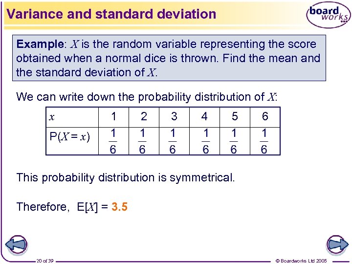
Variance and standard deviation Example: X is the random variable representing the score obtained when a normal dice is thrown. Find the mean and the standard deviation of X. We can write down the probability distribution of X: x 1 2 3 4 5 6 P(X = x) This probability distribution is symmetrical. Therefore, E[X] = 3. 5 20 of 39 © Boardworks Ltd 2005
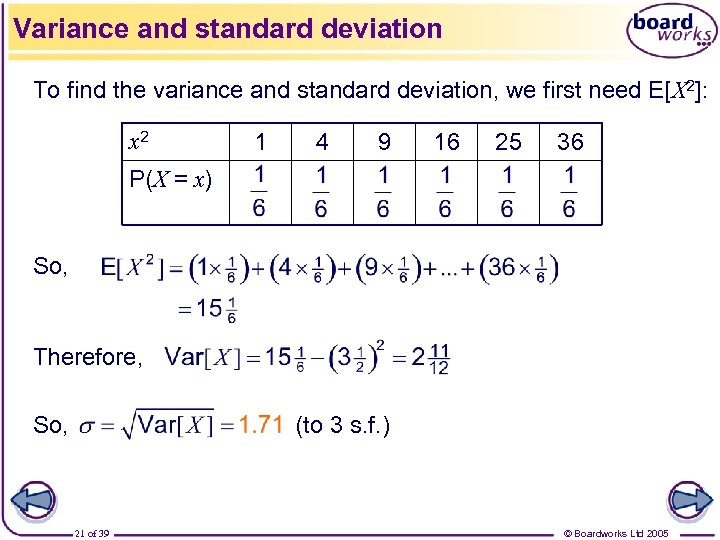
Variance and standard deviation To find the variance and standard deviation, we first need E[X 2]: x 2 1 4 9 16 25 36 P(X = x) So, Therefore, So, (to 3 s. f. ) 21 of 39 © Boardworks Ltd 2005
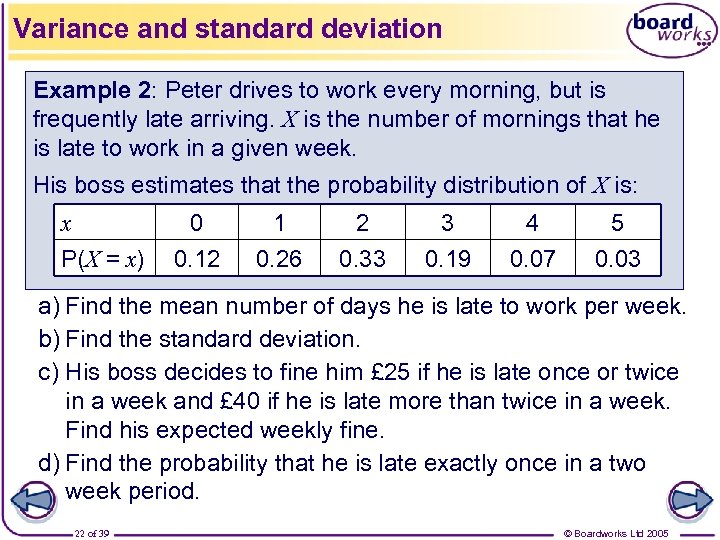
Variance and standard deviation Example 2: Peter drives to work every morning, but is frequently late arriving. X is the number of mornings that he is late to work in a given week. His boss estimates that the probability distribution of X is: x P(X = x) 0 0. 12 1 0. 26 2 0. 33 3 0. 19 4 0. 07 5 0. 03 a) Find the mean number of days he is late to work per week. b) Find the standard deviation. c) His boss decides to fine him £ 25 if he is late once or twice in a week and £ 40 if he is late more than twice in a week. Find his expected weekly fine. d) Find the probability that he is late exactly once in a two week period. 22 of 39 © Boardworks Ltd 2005
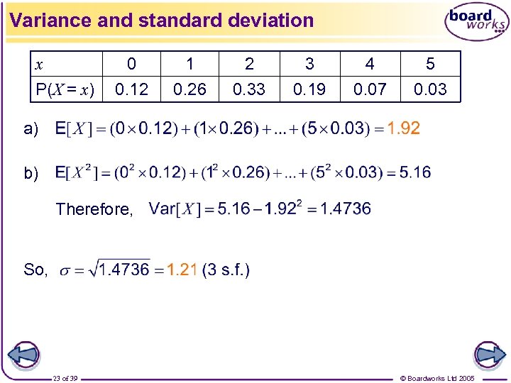
Variance and standard deviation x P(X = x) 0 0. 12 1 0. 26 2 0. 33 3 0. 19 4 0. 07 5 0. 03 a) b) Therefore, So, 23 of 39 © Boardworks Ltd 2005
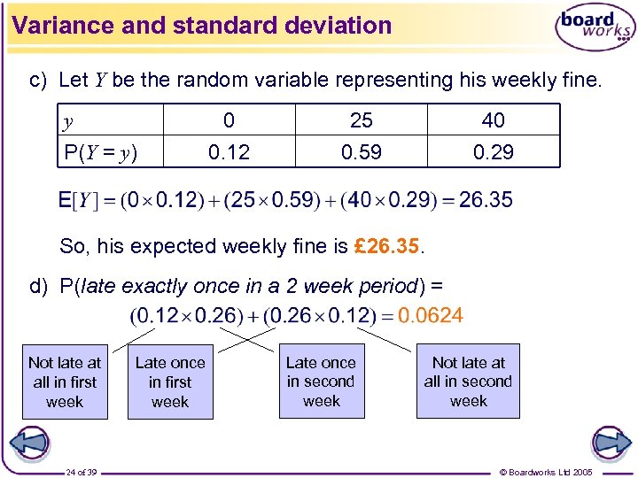
Variance and standard deviation c) Let Y be the random variable representing his weekly fine. y P(Y = y) 0 0. 12 25 0. 59 40 0. 29 So, his expected weekly fine is £ 26. 35. d) P(late exactly once in a 2 week period) = Not late at all in first week 24 of 39 Late once in first week Late once in second week Not late at all in second week © Boardworks Ltd 2005
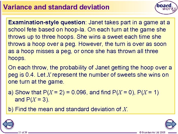
Variance and standard deviation Examination-style question: Janet takes part in a game at a school fete based on hoop-la. On each turn at the game she throws up to three hoops. She wins a sweet each time she throws a hoop over a peg. However, the turn is over as soon as a hoop misses a peg, or once she has thrown all three hoops. On each throw, the probability of Janet getting the hoop over a peg is 0. 4. Let X represent the number of sweets she wins on one turn at the game. a) Show that P(X = 2) = 0. 096, and find P(X = 0), P(X = 1) and P(X = 3). b) Find the mean and standard deviation of X. 25 of 39 © Boardworks Ltd 2005
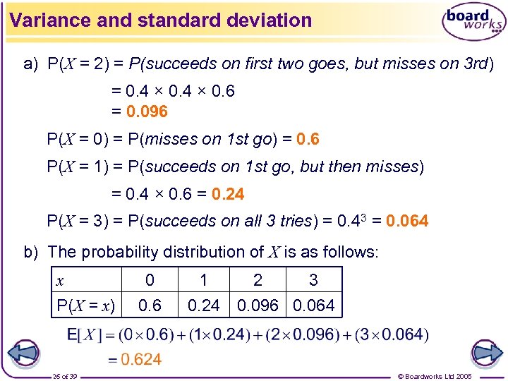
Variance and standard deviation a) P(X = 2) = P(succeeds on first two goes, but misses on 3 rd) = 0. 4 × 0. 6 = 0. 096 P(X = 0) = P(misses on 1 st go) = 0. 6 P(X = 1) = P(succeeds on 1 st go, but then misses) = 0. 4 × 0. 6 = 0. 24 P(X = 3) = P(succeeds on all 3 tries) = 0. 43 = 0. 064 b) The probability distribution of X is as follows: x P(X = x) 26 of 39 0 0. 6 1 2 3 0. 24 0. 096 0. 064 © Boardworks Ltd 2005
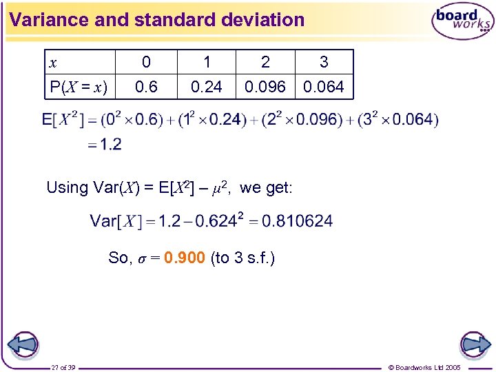
Variance and standard deviation x P(X = x) 0 0. 6 1 0. 24 2 0. 096 3 0. 064 Using Var(X) = E[X 2] – μ 2, we get: So, σ = 0. 900 (to 3 s. f. ) 27 of 39 © Boardworks Ltd 2005
Discrete uniform distribution Introduction to discrete random variables Contents Cumulative distribution functions Expectation Variance and standard deviation for random variables Discrete uniform distribution Expectation algebra – some key results 28 of 39 © Boardworks Ltd 2005
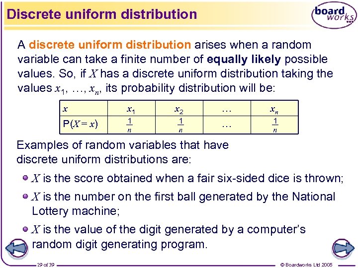
Discrete uniform distribution A discrete uniform distribution arises when a random variable can take a finite number of equally likely possible values. So, if X has a discrete uniform distribution taking the values x 1, …, xn, its probability distribution will be: x P(X = x) x 1 x 2 … xn … Examples of random variables that have discrete uniform distributions are: X is the score obtained when a fair six-sided dice is thrown; X is the number on the first ball generated by the National Lottery machine; X is the value of the digit generated by a computer’s random digit generating program. 29 of 39 © Boardworks Ltd 2005
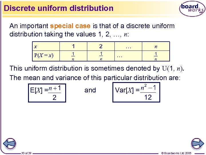
Discrete uniform distribution An important special case is that of a discrete uniform distribution taking the values 1, 2, …, n: x 1 2 P(X = x) … n … This uniform distribution is sometimes denoted by U(1, n). The mean and variance of this particular distribution are: E[X] = 30 of 39 and Var[X] = © Boardworks Ltd 2005
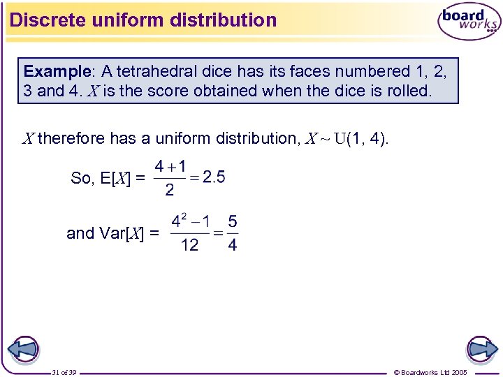
Discrete uniform distribution Example: A tetrahedral dice has its faces numbered 1, 2, 3 and 4. X is the score obtained when the dice is rolled. X therefore has a uniform distribution, X ~ U(1, 4). So, E[X] = and Var[X] = 31 of 39 © Boardworks Ltd 2005
Expectation algebra Introduction to discrete random variables Contents Cumulative distribution functions Expectation Variance and standard deviation for random variables Discrete uniform distribution Expectation algebra – some key results 32 of 39 © Boardworks Ltd 2005
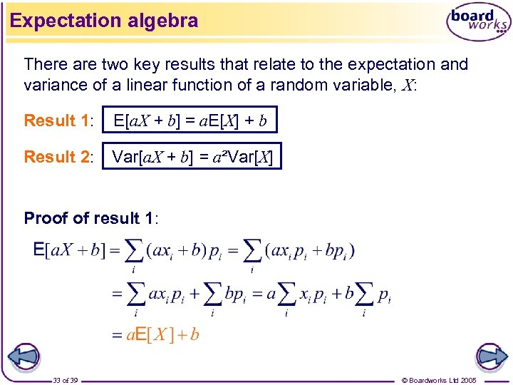
Expectation algebra There are two key results that relate to the expectation and variance of a linear function of a random variable, X: Result 1: E[a. X + b] = a. E[X] + b Result 2: Var[a. X + b] = a²Var[X] Proof of result 1: 33 of 39 © Boardworks Ltd 2005
![Expectation algebra Result 2: Var[a. X + b] = a²Var[X] Proof of result 2: Expectation algebra Result 2: Var[a. X + b] = a²Var[X] Proof of result 2:](https://present5.com/presentation/17d787c278d464cee7215813df315d3a/image-34.jpg)
Expectation algebra Result 2: Var[a. X + b] = a²Var[X] Proof of result 2: Remember: where μ = E[X] 34 of 39 © Boardworks Ltd 2005
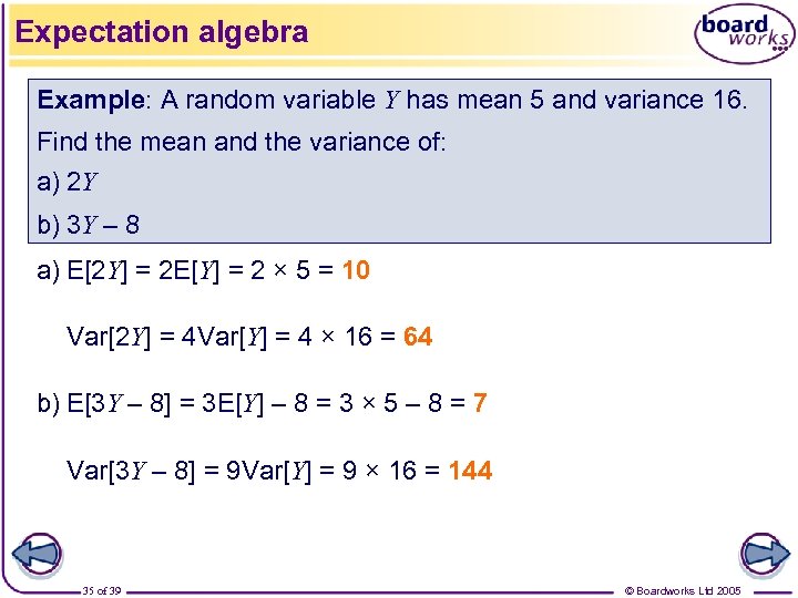
Expectation algebra Example: A random variable Y has mean 5 and variance 16. Find the mean and the variance of: a) 2 Y b) 3 Y – 8 a) E[2 Y] = 2 E[Y] = 2 × 5 = 10 Var[2 Y] = 4 Var[Y] = 4 × 16 = 64 b) E[3 Y – 8] = 3 E[Y] – 8 = 3 × 5 – 8 = 7 Var[3 Y – 8] = 9 Var[Y] = 9 × 16 = 144 35 of 39 © Boardworks Ltd 2005
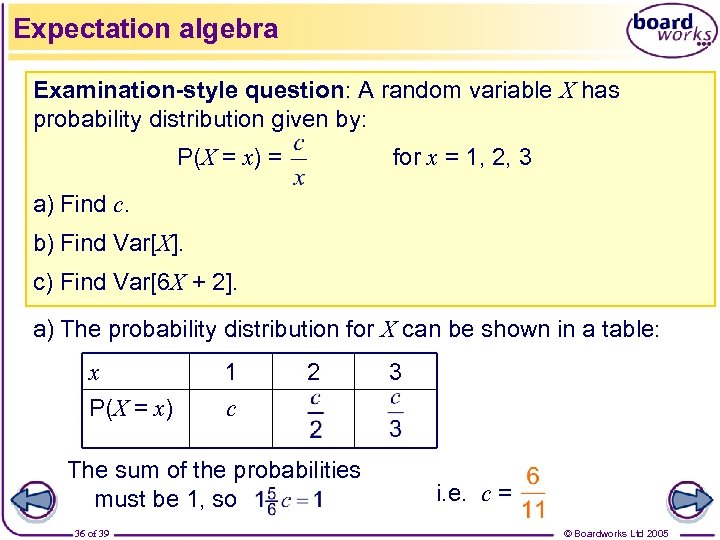
Expectation algebra Examination-style question: A random variable X has probability distribution given by: P(X = x) = for x = 1, 2, 3 a) Find c. b) Find Var[X]. c) Find Var[6 X + 2]. a) The probability distribution for X can be shown in a table: x P(X = x) 1 c 2 The sum of the probabilities must be 1, so 36 of 39 3 i. e. c = © Boardworks Ltd 2005
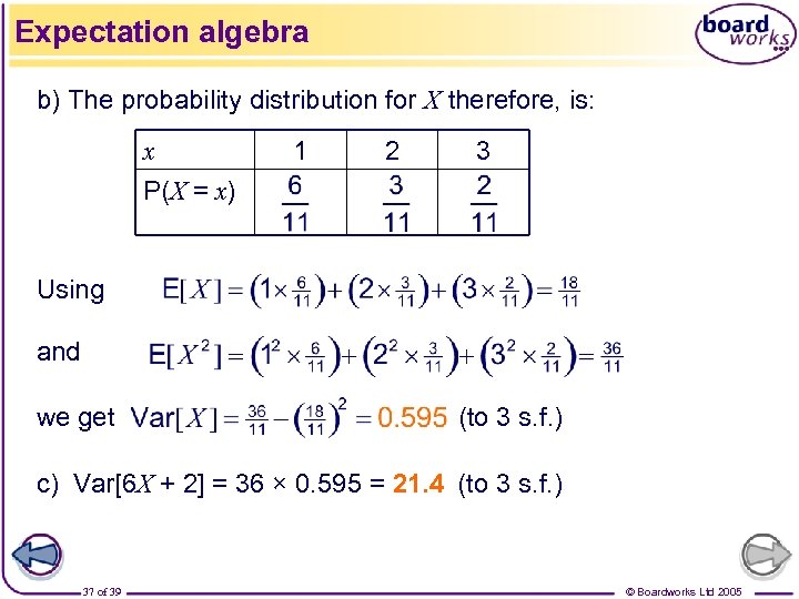
Expectation algebra b) The probability distribution for X therefore, is: x P(X = x) 1 2 3 Using and we get (to 3 s. f. ) c) Var[6 X + 2] = 36 × 0. 595 = 21. 4 (to 3 s. f. ) 37 of 39 © Boardworks Ltd 2005
17d787c278d464cee7215813df315d3a.ppt