I AD AS Model To Analyze changes in

I. AD/AS Model • To Analyze changes in real GDP & price level simultaneously • Provides insights on inflation, unemployment, & economic growth • Aggregate Demand – Amounts of real output – Buyers collectively desire – At each possible price level • Aggregate Supply – Levels of real domestic output firms will produce – At each possible price level

II. Aggregate Demand Curve • Income & substitution effects do not apply • AD Curve – negative slope – Real-Balances effect • Higher price level means real value of savings decreases • Thus lowering consumption – Interest-rate effect • High demand for $ leads to high interest rates • High interest rates limit investment spending • Thus leads to less real output – Foreign purchases effect • US price level up then foreigners buy less US goods

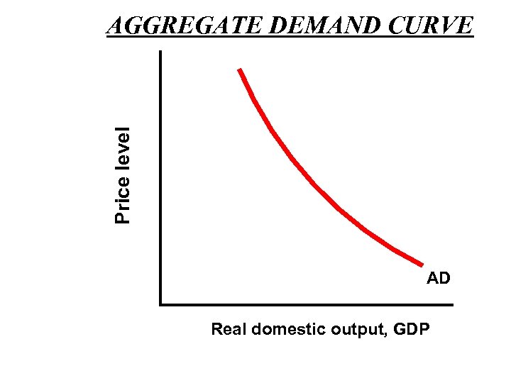Price level AGGREGATE DEMAND CURVE AD Real domestic output, GDP

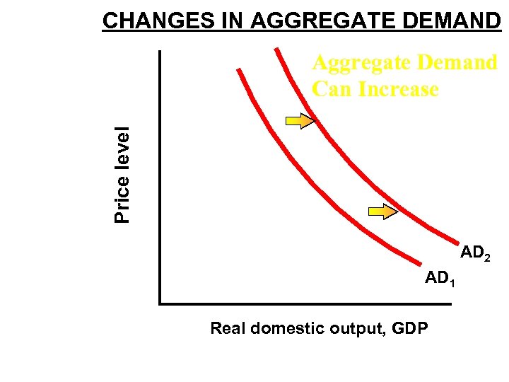CHANGES IN AGGREGATE DEMAND Price level Aggregate Demand Can Increase AD 2 AD 1 Real domestic output, GDP

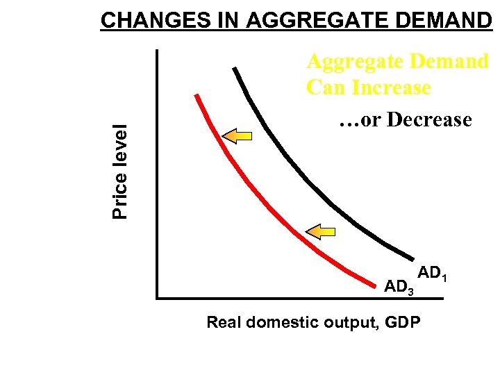Price level CHANGES IN AGGREGATE DEMAND Aggregate Demand Can Increase …or Decrease AD 3 AD 1 Real domestic output, GDP

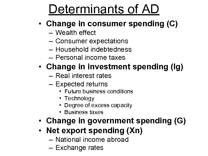Determinants of AD • Change in consumer spending (C) – – Wealth effect Consumer expectations Household indebtedness Personal income taxes • Change in investment spending (Ig) – Real interest rates – Expected returns • • Future business conditions Technology Degree of excess capacity Business taxes • Change in government spending (G) • Net export spending (Xn) – National income abroad – Exchange rates

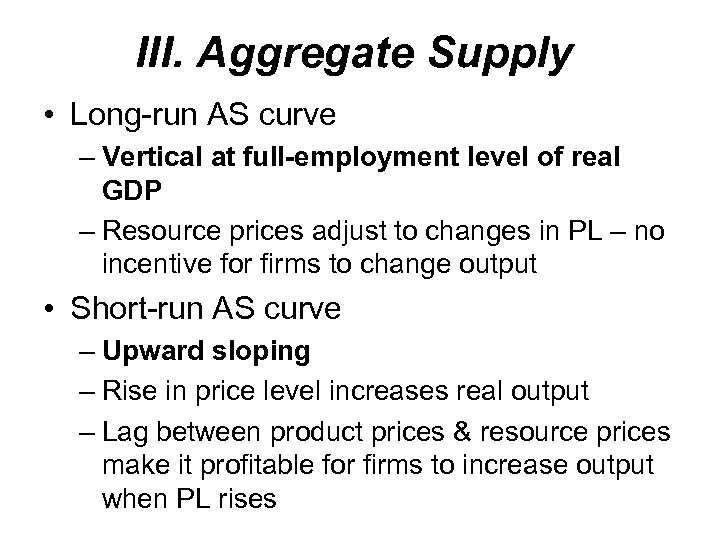III. Aggregate Supply • Long-run AS curve – Vertical at full-employment level of real GDP – Resource prices adjust to changes in PL – no incentive for firms to change output • Short-run AS curve – Upward sloping – Rise in price level increases real output – Lag between product prices & resource prices make it profitable for firms to increase output when PL rises

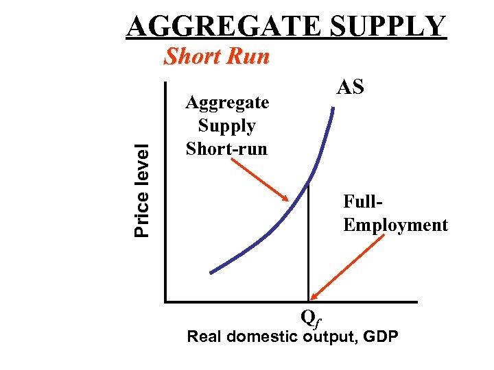AGGREGATE SUPPLY Price level Short Run AS Aggregate Supply Short-run Full. Employment Qf Real domestic output, GDP

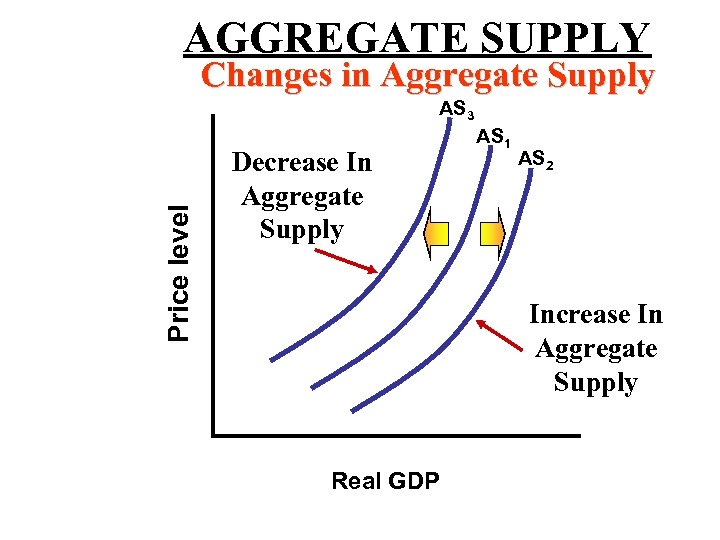AGGREGATE SUPPLY Changes in Aggregate Supply Price level AS 3 Decrease In Aggregate Supply AS 1 AS 2 Increase In Aggregate Supply Real GDP

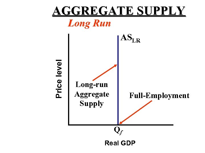AGGREGATE SUPPLY Long Run Price level ASLR Long-run Aggregate Supply Full-Employment Qf Real GDP

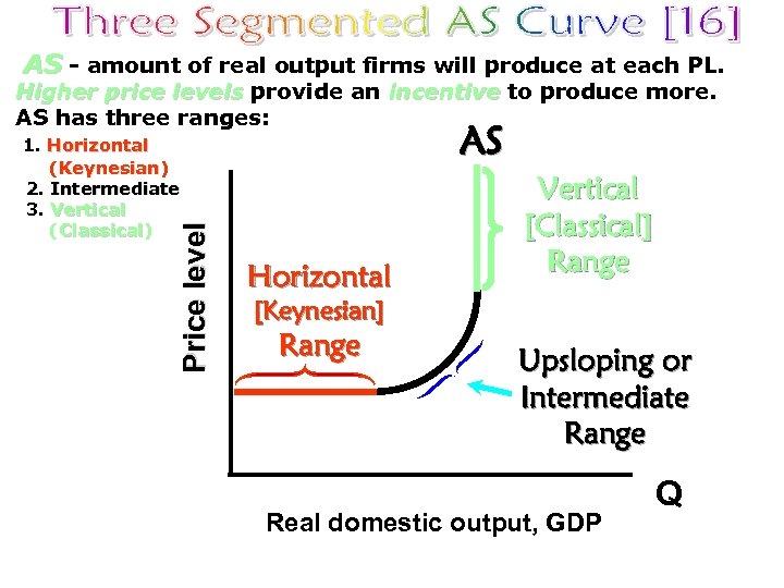AS - amount of real output firms will produce at each PL. Higher price levels provide an incentive to produce more. AS has three ranges: AS Price level 1. Horizontal (Keynesian) Keynesian 2. Intermediate 3. Vertical (Classical) Classical Horizontal Vertical [Classical] Range [Keynesian] Range Upsloping or Intermediate Range Real domestic output, GDP Q

IV. Determinants of AS • Input prices – Domestic • Land • Labor • Capital – Prices of imported resources – Market power (OPEC)

• Productivity = Total output/total inputs • Legal-institutional environment – Business taxes and subsidies – Government regulation

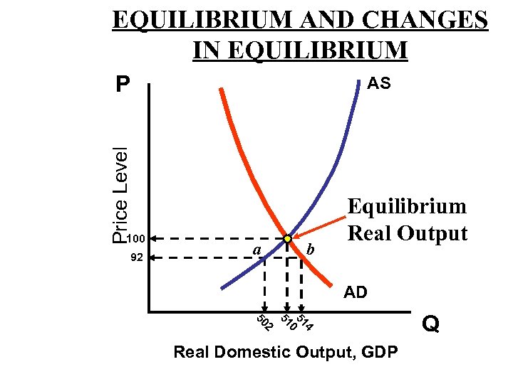EQUILIBRIUM AND CHANGES IN EQUILIBRIUM Price Level P 100 92 AS a b Equilibrium Real Output AD 4 51 0 51 2 50 Real Domestic Output, GDP Q

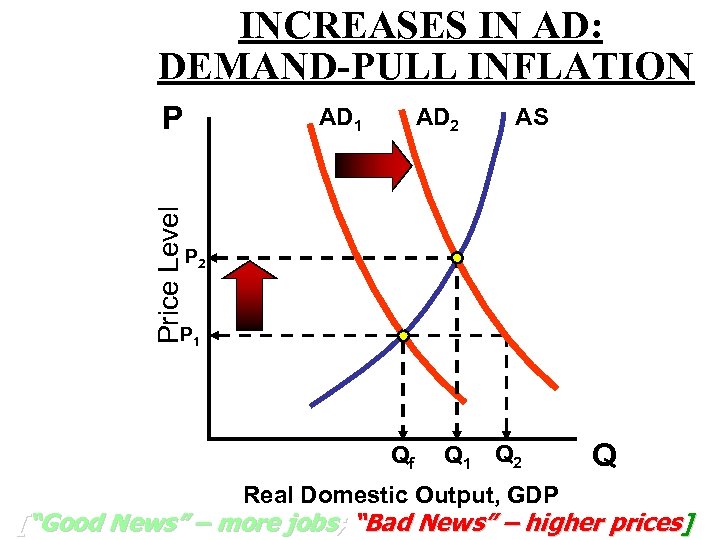INCREASES IN AD: DEMAND-PULL INFLATION Price Level P AD 1 AD 2 AS P 2 P 1 Qf Q 1 Q 2 Real Domestic Output, GDP Q [“Good News” – more jobs; “Bad News” – higher prices]

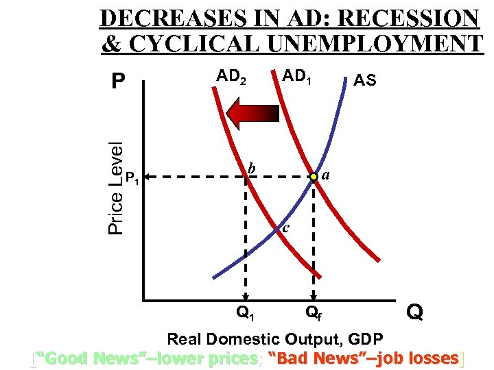DECREASES IN AD: RECESSION & CYCLICAL UNEMPLOYMENT Price Level P P 1 AD 2 AD 1 b AS a c Q 1 Qf Q Real Domestic Output, GDP [“Good News”–lower prices; “Bad News”–job losses]

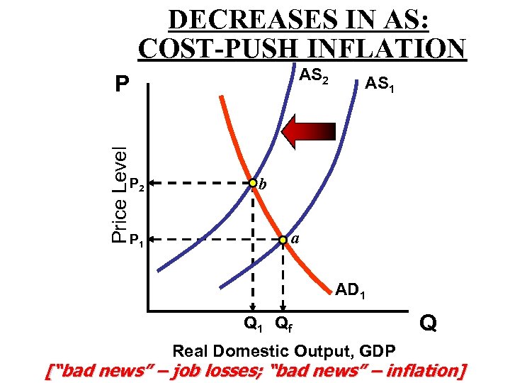DECREASES IN AS: COST-PUSH INFLATION AS 2 Price Level P P 2 P 1 AS 1 b a AD 1 Qf Real Domestic Output, GDP Q [“bad news” – job losses; “bad news” – inflation]

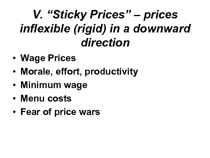V. “Sticky Prices” – prices inflexible (rigid) in a downward direction • • • Wage Prices Morale, effort, productivity Minimum wage Menu costs Fear of price wars

Consumption Investment Gov. Spending Exports Injections Full Employment [Frictional & structural] Income Employment Output Saving Taxes Imports *Classicals – “A leakage down the drain of saving is returned thru the spigot of investment. ” Leakages An economy in equilibrium at FE

Review of the Marginal Propensities 1. If consumption increases from 465 to 480 and disposable income increases from 490 to 510. What is the marginal propensity to consume? 15/20 =. 75 2. If the marginal propensity to consume is 0. 8 then what is the marginal propensity to save? MPS = 0. 2 3. Why will the MPC + MPS always equal Consuming or saving is an either-or proposition 1?

Aggregate Expenditures Model

Building [Simple [Basic] economy to Complex economy] [C + Ig] Private-closed Private - closed [C + Ig + Xn] Private-open (AE 3)630 (AE 2)550 (AE 1)470 C=390 G +20 n +20 X Ig +20 Mixed - open Mixed-open AE 3 (C+Ig+G+Xn) (Complex Economy) [Mixed-open] AE 2 (C+Ig+Xn) (Private-open) [X(40)-M(20)] AE 1(C+Ig)[Basic Economy][Private(no G)-Closed(no X or M)] AE(C+Ig+G) Consumption +80 +80 0 390 470 550 630 Real GDP “Mult” = 4 AE(C+Ig+G) [C+Ig+G+Xn] Private-open AE(C+Ig 1) 10 G 460 YR 500 Real GDP Y*

I. AE Model / Keynesian Cross Model • Aggregate Expenditures means total spending • When AE fall – Total output & employment decrease • When AE rise – Total output & employment increase

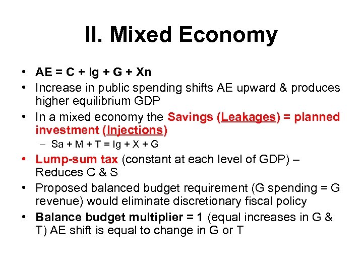II. Mixed Economy • AE = C + Ig + G + Xn • Increase in public spending shifts AE upward & produces higher equilibrium GDP • In a mixed economy the Savings (Leakages) = planned investment (Injections) – Sa + M + T = Ig + X + G • Lump-sum tax (constant at each level of GDP) – Reduces C & S • Proposed balanced budget requirement (G spending = G revenue) would eliminate discretionary fiscal policy • Balance budget multiplier = 1 (equal increases in G & T) AE shift is equal to change in G or T

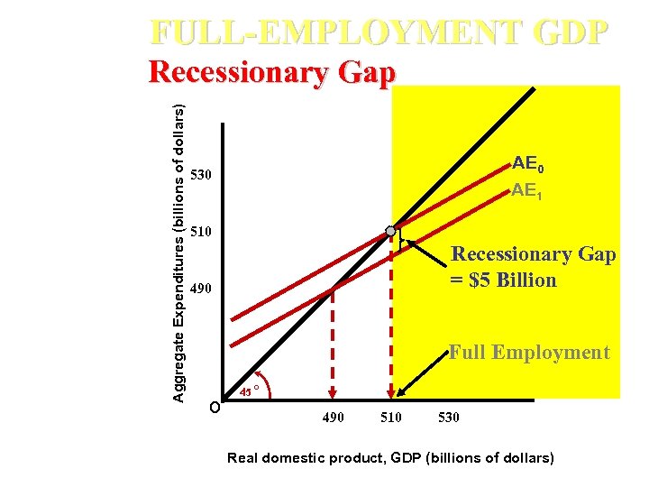FULL-EMPLOYMENT GDP Aggregate Expenditures (billions of dollars) Recessionary Gap AE 0 AE 1 530 510 Recessionary Gap = $5 Billion 490 Full Employment o 45 o 490 510 530 Real domestic product, GDP (billions of dollars)

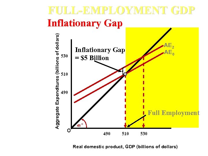FULL-EMPLOYMENT GDP Aggregate Expenditures (billions of dollars) Inflationary Gap 530 AE 2 AE 0 Inflationary Gap = $5 Billion 510 490 Full Employment o 45 o 490 510 530 Real domestic product, GDP (billions of dollars)

III. Limitations • No price-level changes • Ignores premature demand-pull inflation • Limits real GDP to the full-employment level of output • Ignores cost-push inflation • Does not allow for self-correction