

3db2150f6bcb195bfa59e1ccfc2ddeb0.ppt
- Количество слайдов: 65
 I 256: Applied Natural Language Processing Marti Hearst Nov 6, 2006
 2") Today Text Clustering Latent Semantic Indexing (LSA) 2
Today Text Clustering Latent Semantic Indexing (LSA) 2
 Text Clustering Finds overall similarities among groups of documents Finds overall similarities among groups of tokens Picks out some themes, ignores others 3
 Text Clustering is “The art of finding groups in data. ” -- Kaufmann and Rousseeu Term 1 Term 2 4
 Text Clustering is “The art of finding groups in data. ” -- Kaufmann and Rousseeu Term 1 Term 2 5
 Clustering Applications Find semantically related words by combining similarity evidence from multiple indicators Try to find overall trends or patterns in text collections Slide by Vasileios Hatzivassiloglou 6
 “Training” in Clustering is an unsupervised learning method For each data set, a totally fresh solution is constructed Therefore, there is no training However, we often use some data for which we have additional information on how it should be partitioned to evaluate the performance of the clustering method Slide by Vasileios Hatzivassiloglou 7
 Pair-wise Document Similarity nova A B C D galaxy 5 film role 1 5 4 3 h’wood 2 1 heat diet fur 1 1 2 How to compute document similarity? 8
 nova A B C D galaxy 1") Pair-wise Document Similarity (no normalization for simplicity) nova A B C D galaxy 1 3 5 heat h’wood film role 2 1 5 4 diet fur 1 1 2 9
Pair-wise Document Similarity (no normalization for simplicity) nova A B C D galaxy 1 3 5 heat h’wood film role 2 1 5 4 diet fur 1 1 2 9
 10") Pair-wise Document Similarity (cosine normalization) 10
Pair-wise Document Similarity (cosine normalization) 10
 Document/Document Matrix 11
 Hierarchical clustering methods Agglomerative or bottom-up: Start with each sample in its own cluster Merge the two closest clusters Repeat until one cluster is left Divisive or top-down: Start with all elements in one cluster Partition one of the current clusters in two Repeat until all samples are in singleton clusters Slide by Vasileios Hatzivassiloglou 12
 Agglomerative Clustering A B C D E F G H I 13
 Agglomerative Clustering A B C D E F G H I 14
 Agglomerative Clustering A B C D E F G H I 15
 Merging Nodes Each node is a combination of the documents combined below it We represent the merged nodes as a vector of term weights This vector is referred to as the cluster centroid Slide by Vasileios Hatzivassiloglou 16
 Merging criteria We need to extend the distance measure from samples to sets of samples The complete linkage method The single linkage method The average linkage method Slide by Vasileios Hatzivassiloglou 17
 Single-link merging criteria merge each word type is a single-point cluster Merge closest pair of clusters: Single-link: clusters are close if any of their points are dist(A, B) = min dist(a, b) for a A, b B 18
 Bottom-Up Clustering – Single-Link Fast, but tend to get long, stringy, meandering clusters . . . 19
 Bottom-Up Clustering – Complete-Link distance between clusters Again, merge closest pair of clusters: Complete-link: clusters are close only if all of their points are dist(A, B) = max dist(a, b) for a A, b B 20
 Bottom-Up Clustering – Complete-Link distance between clusters Slow to find closest pair – need quadratically many distances 21
 K-Means Clustering Decide on a pair-wise similarity measure 2 Find K centers using agglomerative clustering 1 take a small sample group bottom up until K groups found 3 Assign each document to nearest center, forming new clusters 4 Repeat 3 as necessary 22
 k-Medians Similar to k-means but instead of calculating the means across features, it selects as ci the sample in cluster Ci that minimizes (the median) Advantages Does not require feature vectors Distance between samples is always available Statistics with medians are more robust than statistics with means Slide by Vasileios Hatzivassiloglou 23
 Choosing k In both hierarchical and k-means/medians, we need to be told where to stop, i. e. , how many clusters to form This is partially alleviated by visual inspection of the hierarchical tree (the dendrogram) It would be nice if we could find an optimal k from the data We can do this by trying different values of k and seeing which produces the best separation among the resulting clusters. Slide by Vasileios Hatzivassiloglou 24
 Scatter/Gather: Clustering a Large Text Collection Cutting, Pedersen, Tukey & Karger 92, 93 Hearst & Pedersen 95 Cluster sets of documents into general “themes”, like a table of contents Display the contents of the clusters by showing topical terms and typical titles User chooses subsets of the clusters and re-clusters the documents within Resulting new groups have different “themes” 25
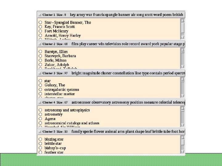
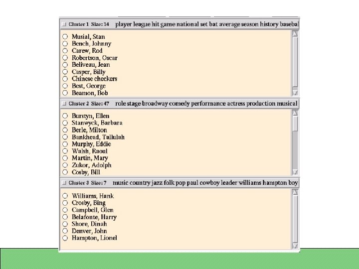
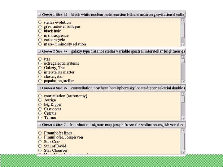
 97") S/G Example: query on “star” Encyclopedia text 8 symbols 68 film, tv (p) 97 astrophysics 67 astronomy(p) 10 flora/fauna 14 sports 47 film, tv 7 music 12 steller phenomena 49 galaxies, stars 29 constellations 7 miscelleneous Clustering and re-clustering is entirely automated 26
S/G Example: query on “star” Encyclopedia text 8 symbols 68 film, tv (p) 97 astrophysics 67 astronomy(p) 10 flora/fauna 14 sports 47 film, tv 7 music 12 steller phenomena 49 galaxies, stars 29 constellations 7 miscelleneous Clustering and re-clustering is entirely automated 26
 Clustering Retrieval Results Tends to place similar docs together So can be used as a step in relevance ranking But not great for showing to users Exception: good for showing what to throw out! 30
 Another use of clustering Use clustering to map the entire huge multidimensional document space into a huge number of small clusters. “Project” these onto a 2 D graphical representation Looks neat, but doesn’t work well as an information retrieval interface. 31
 32") Clustering Multi-Dimensional Document Space (image from Wise et al 95) 32
Clustering Multi-Dimensional Document Space (image from Wise et al 95) 32
 How to evaluate clusters? In practice, it’s hard to do Different algorithms’ results look good and bad in different ways It’s difficult to distinguish their outcomes In theory, define an evaluation function Typically choose something easy to measure (e. g. , the sum of the average distance in each class) 33
 Two Types of Document Clustering Grouping together of “similar” objects Hard Clustering -- Each object belongs to a single cluster Soft Clustering -- Each object is probabilistically assigned to clusters Slide by Inderjit S. Dhillon 34
 Soft clustering A variation of many clustering methods Instead of assigning each data sample to one and only one cluster, it calculates probabilities of membership for all clusters So, a sample might belong to cluster A with probability 0. 4 and to cluster B with probability 0. 6 Slide by Vasileios Hatzivassiloglou 35
 Application: Clustering of adjectives Cluster adjectives based on the nouns they modify Multiple syntactic clues for modification The similarity measure is Kendall’s τ, a robust measure of similarity Clustering is done via a hill-climbing method that minimizes the combined average dissimilarity Predicting the semantic orientation of adjectives, V Hatzivassiloglou, KR Mc. Keown, EACL 1997 Slide by Vasileios Hatzivassiloglou 36
 Clustering of nouns Work by Pereira, Tishby, and Lee Dissimilarity is KL divergence Asymmetric relationship: nouns are clustered, verbs which have the nouns as objects serve as indicators Soft, hierarchical clustering Slide by Vasileios Hatzivassiloglou 37
 Distributional Clustering of English Words - Pereira, Tishby and Lee, ACL 93
 Distributional Clustering of English Words - Pereira, Tishby and Lee, ACL 93
 Latent Semantic Analysis Mathematical/statistical technique for extracting and representing the similarity of meaning of words Represents word and passage meaning as highdimensional vectors in the semantic space Uses Singular Value Decomposition (SVD) to simulate human learning of word and passage meaning Its success depends on: Sufficient scale and sampling of the data it is given Choosing the right number of dimensions to extract Slide by Kostas Kleisouris 40
 LSA Characteristics Why is reducing dimensionality beneficial? Some words with similar occurrence patterns are projected onto the same dimension Closely mimics human judgments of meaning similarity Slide by Schone, Jurafsky, and Stenchikova 41
 Sample Applications of LSA Essay Grading LSA is trained on a large sample of text from the same domain as the topic of the essay Each essay is compared to a large set of essays scored by experts and a subset of the most similar identified by LSA The target essay is assigned a score consisting of a weighted combination of the scores for the comparison essays Slide by Kostas Kleisouris 42
 Sample Applications of LSA Prediction of differences in comprehensibility of texts By using conceptual similarity measures between successive sentences LSA has predicted comprehension test results with students Evaluate and give advice to students as they write and revise summaries of texts they have read Assess psychiatric status By representing the semantic content of answers to psychiatric interview questions Slide by Kostas Kleisouris 43
 Sample Applications of LSA Improving Information Retrieval Use LSA to match users’ queries with documents that have the desired conceptual meaning Not used in practice – doesn’t help much when you have large corpora to match against, but maybe helpful for a few difficult queries and for term expansion Slide by Kostas Kleisouris 44
 LSA intuitions Implements the idea that the meaning of a passage is the sum of the meanings of its words: meaning of word 1 + meaning of word 2 + … + meaning of wordn = meaning of passage This “bag of words” function shows that a passage is considered to be an unordered set of word tokens and the meanings are additive. By creating an equation of this kind for every passage of language that a learner observes, we get a large system of linear equations. Slide by Kostas Kleisouris 45
 LSA Intuitions However Too few equations to specify the values of the variables Different values for the same variable (natural since meanings are vague or multiple) Instead of finding absolute values for the meanings, they are represented in a richer form (vectors) Use of SVD (reduces the linear system into multidimensional vectors) Slide by Kostas Kleisouris 46
 Latent Semantic Analysis A trick from Information Retrieval Each document in corpus is a length-k vector – Or each paragraph, or whatever ed k ar cus don t n bo duct ove dv ba a ar a a ab ab (0, 3, 3, 1, 0, 7, . . . e urgy ot m g zy zy 1, 0) a single document Slide by Jason Eisner 47
 Latent Semantic Analysis A trick from Information Retrieval Each document in corpus is a length-k vector Plot all documents in corpus Reduced-dimensionality plot Slide by Jason Eisner True plot in k dimensions 48
 Latent Semantic Analysis Reduced plot is a perspective drawing of true plot It projects true plot onto a few axes a best choice of axes – shows most variation in the data. Found by linear algebra: “Singular Value Decomposition” (SVD) Reduced-dimensionality plot Slide by Jason Eisner True plot in k dimensions 49
 Latent Semantic Analysis SVD plot allows best possible reconstruction of true plot (i. e. , can recover 3 -D coordinates with minimal distortion) Ignores variation in the axes that it didn’t pick out Hope that variation’s just noise and we want to ignore it True plot in k dimensions theme A Slide by Jason Eisner theme word 2 theme B B Reduced-dimensionality plot theme A d 3 or w word 1 50
 Latent Semantic Analysis SVD finds a small number of theme vectors Approximates each doc as linear combination of themes Coordinates in reduced plot = linear coefficients How much of theme A in this document? How much of theme B? Each theme is a collection of words that tend to appear together theme A Slide by Jason Eisner True plot in k dimensions B theme B Reduced-dimensionality plot 51
: terms 1 2 3 4") Latent Semantic Analysis Another perspective (similar to neural networks): terms 1 2 3 4 5 6 7 8 9 matrix of strengths (how strong is each term in each document? ) 1 2 3 4 5 6 7 documents Slide by Jason Eisner Each connection has a weight given by the matrix. 52
Latent Semantic Analysis Another perspective (similar to neural networks): terms 1 2 3 4 5 6 7 8 9 matrix of strengths (how strong is each term in each document? ) 1 2 3 4 5 6 7 documents Slide by Jason Eisner Each connection has a weight given by the matrix. 52
 Latent Semantic Analysis Which documents is term 5 strong in? terms 1 2 3 4 5 6 7 8 9 docs 2, 5, 6 light up strongest. 1 2 3 4 5 6 7 documents Slide by Jason Eisner 53
 Latent Semantic Analysis Which documents are terms 5 and 8 strong in? terms 1 2 3 4 5 6 7 8 9 This answers a query consisting of terms 5 and 8! 1 2 3 4 5 6 7 documents Slide by Jason Eisner really just matrix multiplication: term vector (query) x strength matrix = doc vector 54
 Latent Semantic Analysis Conversely, what terms are strong in document 5? terms 1 2 3 4 5 6 7 8 9 gives doc 5’s coordinates! 1 2 3 4 5 6 7 documents Slide by Jason Eisner 55
 Latent Semantic Analysis SVD approximates by smaller 3 -layer network Forces sparse data through a bottleneck, smoothing it terms 1 2 3 4 5 6 7 8 9 themes 1 2 3 4 5 6 7 documents Slide by Jason Eisner 1 2 3 4 5 6 7 documents 56
 Latent Semantic Analysis I. e. , smooth sparse data by matrix approx: M A B A encodes camera angle, B gives each doc’s new coords terms 1 2 3 4 5 6 7 8 9 matrix M 1 2 3 4 5 6 7 documents Slide by Jason Eisner A themes B 1 2 3 4 5 6 7 documents 57
 How LSA works Takes as input a corpus of natural language The corpus is parsed into meaningful passages (such as paragraphs) A matrix is formed with passages as rows and words as columns. Cells contain the number of times that a given word is used in a given passage The cell values are transformed into a measure of the information about the passage identity the carry SVD is applied to represent the words and passages as vectors in a high dimensional semantic space Slide by Kostas Kleisouris 58
 Represent text as a matrix documents d 2 d 3 d 4 d 5 d 6 cosmonaut 1 0 0 0 astronaut 0 1 0 0 moon words d 1 1 1 0 0 car 1 0 0 1 1 0 truck 0 0 0 1 A[i, j] = number of of occurrence of a word i in document j Slide by Schone, Jurafsky, and Stenchikova 59
 x S n x") SVD {A}={T}{S}{D}’ m n A m =n T Min(n, m) x S n x m D’ k §Reduce dimensionality to k and compute A 1: m n A 1 k = n T 1 x k k S x k m D’ A 1 is the best least square approximation of A by a matrix in rank k Slide by Schone, Jurafsky, and Stenchikova 60
SVD {A}={T}{S}{D}’ m n A m =n T Min(n, m) x S n x m D’ k §Reduce dimensionality to k and compute A 1: m n A 1 k = n T 1 x k k S x k m D’ A 1 is the best least square approximation of A by a matrix in rank k Slide by Schone, Jurafsky, and Stenchikova 60
 Matrix T T- term matrix. Rows of T correspond to Rows of original matrix A dimensions dim 2 dim 3 dim 4 dim 5 cosmonaut -0. 44 -0. 30 0. 57 0. 58 0. 25 astronaut -0. 13 -0. 33 -0. 59 0. 00 0. 73 moon -0. 48 -0. 51 -0. 37 0. 00 -0. 61 car -0. 70 0. 35 0. 15 -0. 58 0. 16 truck words dim 1 -0. 26 0. 65 -0. 41 0. 58 -0. 09 Dim 2 directly reflects the different co-occurrence patterns Slide by Schone, Jurafsky, and Stenchikova
 correspond to rows") Matrix D’ D- document matrix. Columns of D’ (rows of D) correspond to rows of original matrix A documents d 2 d 3 d 4 d 5 d 6 Dimension 1 dimensions d 1 -0. 75 -0. 28 -0. 20 -0. 45 -0. 33 -0. 12 Dimension 2 -0. 29 -053 -0. 19 0. 63 0. 22 0. 41 Dimension 3 0. 28 -0. 75 0. 45 -0. 20 0. 12 -0. 33 Dimension 4 -0. 00 0. 58 0. 00 -0. 58 Dimension 5 -0. 53 0. 29 0. 63 0. 19 0. 41 -0. 22 Dim 2 directly reflects the different co-occurrence patterns Slide by Schone, Jurafsky, and Stenchikova 62
Matrix D’ D- document matrix. Columns of D’ (rows of D) correspond to rows of original matrix A documents d 2 d 3 d 4 d 5 d 6 Dimension 1 dimensions d 1 -0. 75 -0. 28 -0. 20 -0. 45 -0. 33 -0. 12 Dimension 2 -0. 29 -053 -0. 19 0. 63 0. 22 0. 41 Dimension 3 0. 28 -0. 75 0. 45 -0. 20 0. 12 -0. 33 Dimension 4 -0. 00 0. 58 0. 00 -0. 58 Dimension 5 -0. 53 0. 29 0. 63 0. 19 0. 41 -0. 22 Dim 2 directly reflects the different co-occurrence patterns Slide by Schone, Jurafsky, and Stenchikova 62
 Reevaluating document similarities B = S 1 x D 1 Matrix B is a dimensionality reduction of the original matrix A Compute document correlation B’*B d 1 d 2 d 3 d 4 d 5 d 1 1 d 2 0. 78 1 d 3 0. 40 0. 88 1 d 4 0. 47 -0. 18 -0. 62 1 d 5 0. 74 0. 16 -0. 32 0. 94 1 d 6 0. 10 -0. 54 -0. 87 0. 93 0. 74 d 6 Slide by Schone, Jurafsky, and Stenchikova 1 63
 Unfolding new documents Given a new document, how to determine which documents it is similar to? A = T S D’ T’A = T’ T S D’ T’ A = S D’ q a new vector in the space of A q in reduced space = Slide by Schone, Jurafsky, and Stenchikova T’ * q 64
 Next Time Several takes on blog analysis Sentiment classification 65