f29230dac59df7a6c5be4bc0c05c681c.ppt
- Количество слайдов: 61
Hybrid Control and Switched Systems Lecture #4 Simulation of hybrid systems João P. Hespanha University of California at Santa Barbara
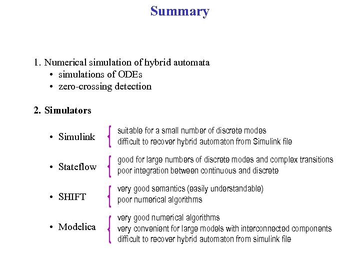
Summary 1. Numerical simulation of hybrid automata • simulations of ODEs • zero-crossing detection 2. Simulators • Simulink • Stateflow • SHIFT • Modelica
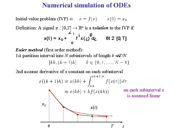
Numerical simulation of ODEs Initial value problem (IVP) ´ Definition: A signal x : [0, T] ! Rn is a solution to the IVP if Euler method (first order method): 1 st partition interval into N subintervals of length h T/N 2 nd assume derivative of x constant on each subinterval x is assumed linear x 0 x(t) 0 T t
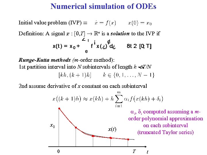
Numerical simulation of ODEs Initial value problem (IVP) ´ Definition: A signal x : [0, T] ! Rn is a solution to the IVP if Runge-Kutta methods (m-order method): 1 st partition interval into N subintervals of length h T/N 2 nd assume derivative of x constant on each subinterval x 0 x(t) 0 ai, di computed assuming a morder polynomial approximation on each subinterval (truncated Taylor series) T t
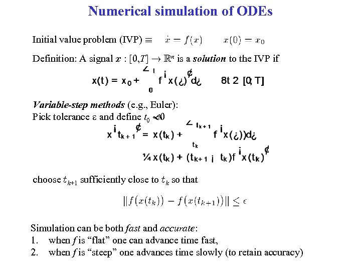
Numerical simulation of ODEs Initial value problem (IVP) ´ Definition: A signal x : [0, T] ! Rn is a solution to the IVP if Variable-step methods (e. g. , Euler): Pick tolerance e and define t 0 0 choose tk+1 sufficiently close to tk so that Simulation can be both fast and accurate: 1. when f is “flat” one can advance time fast, 2. when f is “steep” one advances time slowly (to retain accuracy)
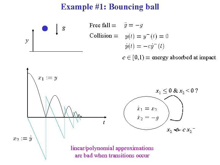
Example #1: Bouncing ball g y Free fall ´ Collision ´ c 2 [0, 1) ´ energy absorbed at impact x 1 · 0 & x 2 < 0 ? t x 2 c x 2 – – linear/polynomial approximations are bad when transitions occur
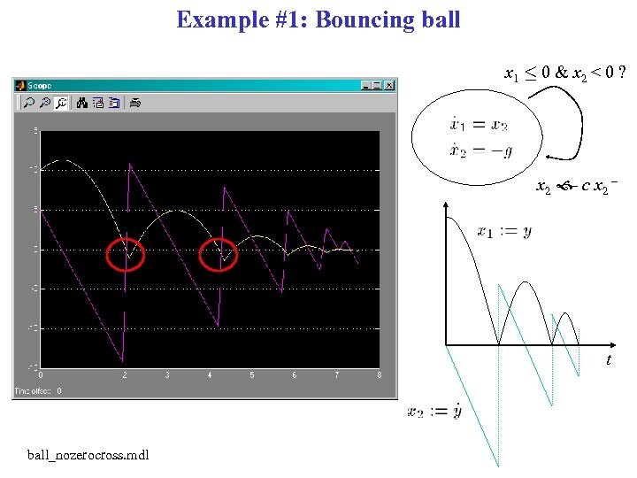
Example #1: Bouncing ball x 1 · 0 & x 2 < 0 ? x 2 c x 2 – – t ball_nozerocross. mdl
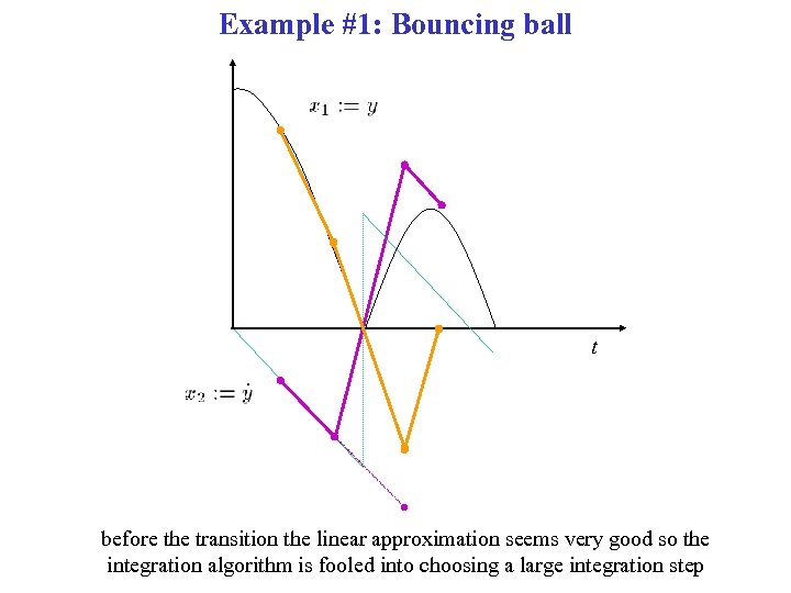
Example #1: Bouncing ball t before the transition the linear approximation seems very good so the integration algorithm is fooled into choosing a large integration step
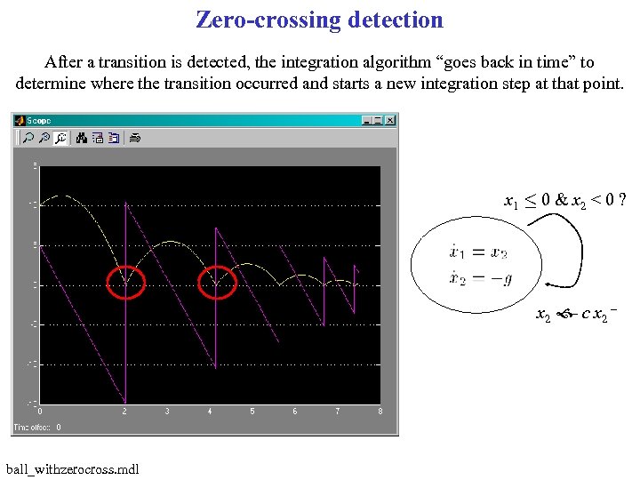
Zero-crossing detection After a transition is detected, the integration algorithm “goes back in time” to determine where the transition occurred and starts a new integration step at that point. x 1 · 0 & x 2 < 0 ? x 2 c x 2 – – ball_withzerocross. mdl
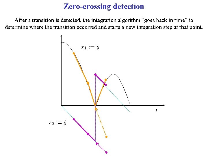
Zero-crossing detection After a transition is detected, the integration algorithm “goes back in time” to determine where the transition occurred and starts a new integration step at that point. t
Summary 1. Numerical simulation of hybrid automata • simulations of ODEs • zero-crossing detection 2. Simulators • Simulink suitable for a small number of discrete modes difficult to recover hybrid automaton from Simulink file • Stateflow good for large numbers of discrete modes and complex transitions poor integration between continuous and discrete • SHIFT very good semantics (easily understandable) poor numerical algorithms • Modelica very good numerical algorithms very convenient for large models with interconnected components difficult to recover hybrid automaton from simulink file
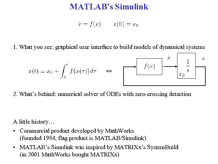
MATLAB’s Simulink 1. What you see: graphical user interface to build models of dynamical systems , 2. What’s behind: numerical solver of ODEs with zero-crossing detection A little history… • Commercial product developed by Math. Works (founded 1984, flag product is MATLAB/Simulink) • MATLAB’s Simulink was inspired by MATRIXx’s System. Build (in 2001 Math. Works bought MATRIXx)
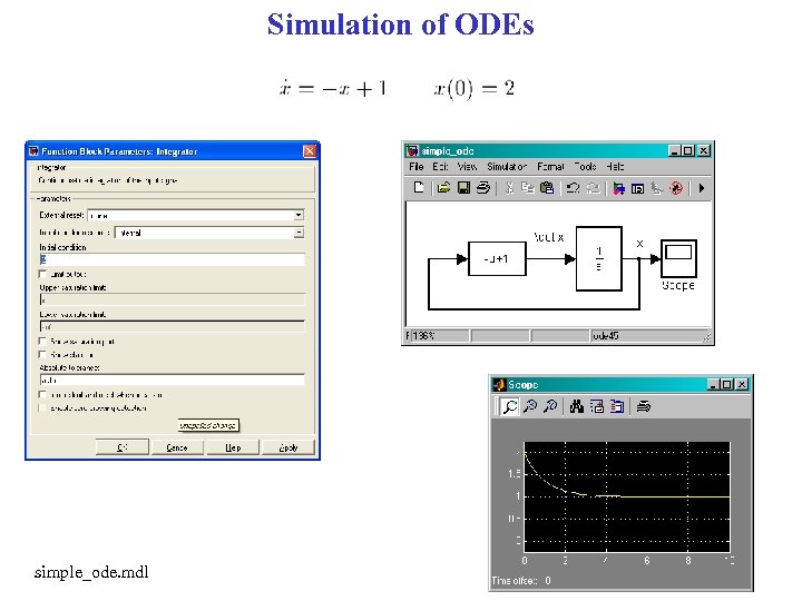
Simulation of ODEs simple_ode. mdl
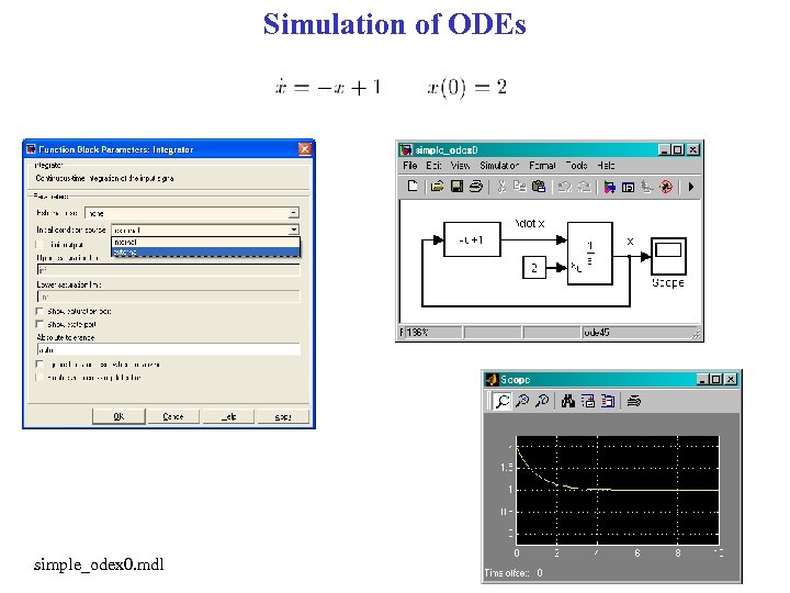
Simulation of ODEs simple_odex 0. mdl
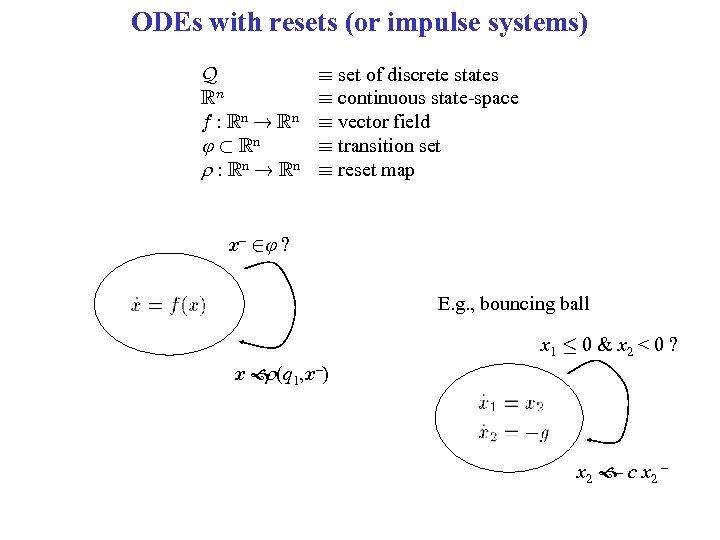
ODEs with resets (or impulse systems) Q Rn f : Rn ! Rn ½ Rn r : Rn ! Rn ´ set of discrete states ´ continuous state-space ´ vector field ´ transition set ´ reset map x – 2 ? E. g. , bouncing ball x 1 · 0 & x 2 < 0 ? x (q 1, x–) r x 2 c x 2 – –
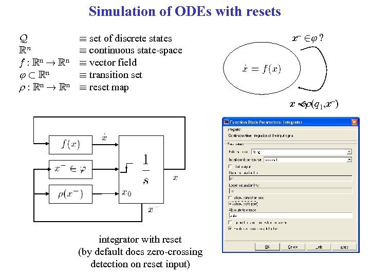
Simulation of ODEs with resets Q Rn f : Rn ! Rn ½ Rn r : Rn ! Rn ´ set of discrete states ´ continuous state-space ´ vector field ´ transition set ´ reset map x – 2 ? x (q 1, x–) r integrator with reset (by default does zero-crossing detection on reset input)
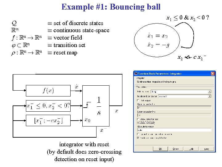
Example #1: Bouncing ball Q Rn f : Rn ! Rn ½ Rn r : Rn ! Rn ´ set of discrete states ´ continuous state-space ´ vector field ´ transition set ´ reset map integrator with reset (by default does zero-crossing detection on reset input) x 1 · 0 & x 2 < 0 ? x 2 c x 2 – –
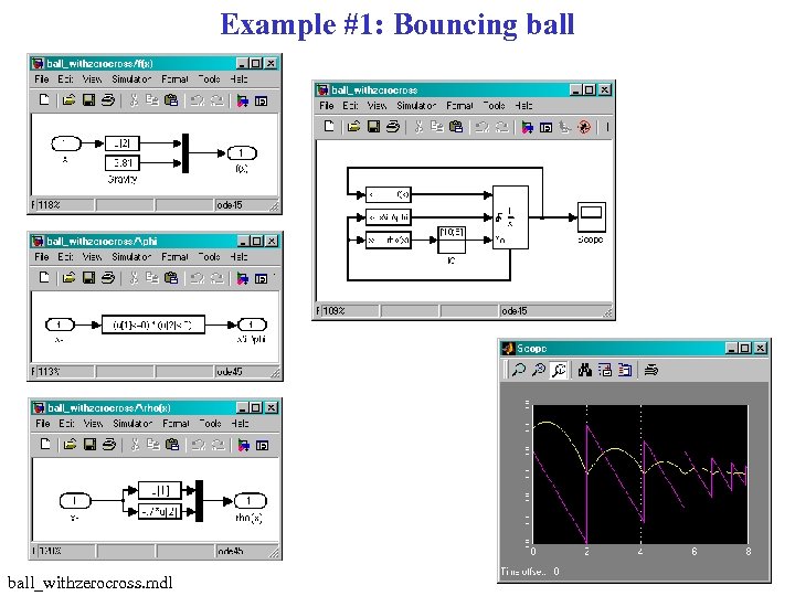
Example #1: Bouncing ball_withzerocross. mdl
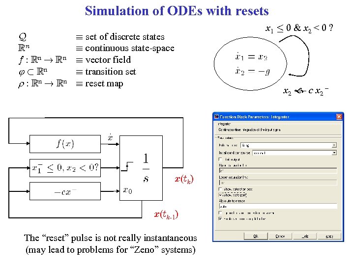
Simulation of ODEs with resets Q Rn f : Rn ! Rn ½ Rn r : Rn ! Rn x 1 · 0 & x 2 < 0 ? ´ set of discrete states ´ continuous state-space ´ vector field ´ transition set ´ reset map x 2 c x 2 – – x(tk) x(tk-1) The “reset” pulse is not really instantaneous (may lead to problems for “Zeno” systems)
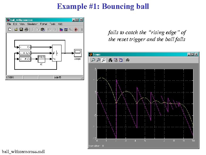
Example #1: Bouncing ball fails to catch the “rising edge” of the reset trigger and the ball falls ball_withzerocross. mdl
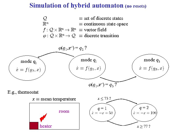
Simulation of hybrid automaton (no resets) Q Rn f : Q £ Rn ! Rn : Q £ Rn ! Q ´ set of discrete states ´ continuous state-space ´ vector field ´ discrete transition (q 1, x–) = q 2 ? mode q 1 mode q 2 mode q 3 (q 1, x–) = q 3 ? E. g. , thermostat x ´ mean temperature room heater x · 73 ? q=1 q=2 x ¸ 77 ?
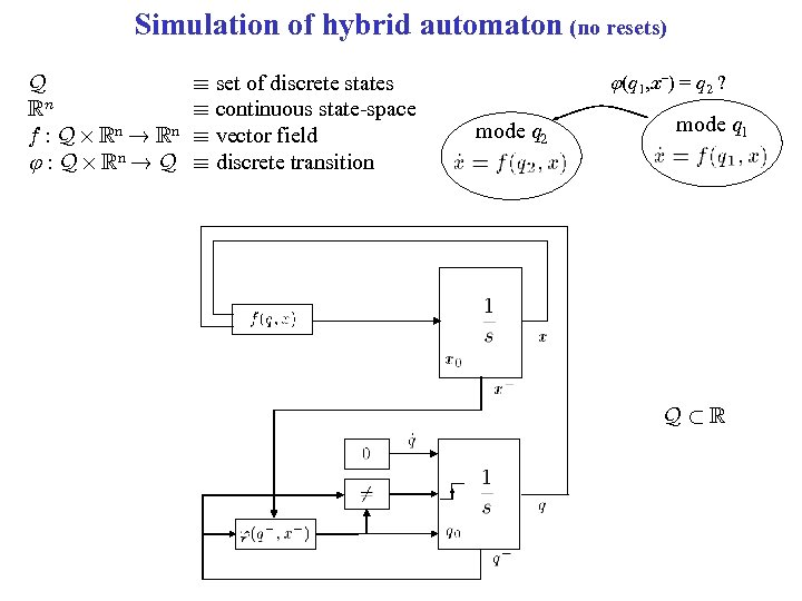
Simulation of hybrid automaton (no resets) Q Rn f : Q £ Rn ! Rn : Q £ Rn ! Q ´ set of discrete states ´ continuous state-space ´ vector field ´ discrete transition (q 1, x–) = q 2 ? mode q 2 mode q 1 Q½R
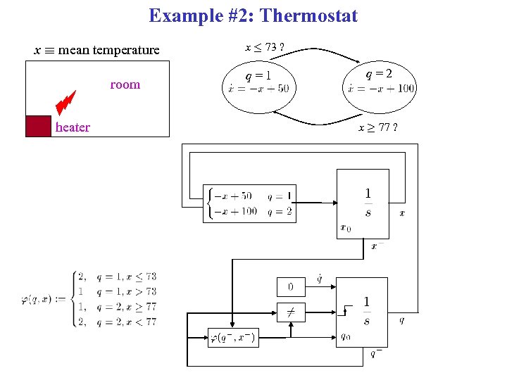
Example #2: Thermostat x ´ mean temperature room heater x · 73 ? q=1 q=2 x ¸ 77 ?
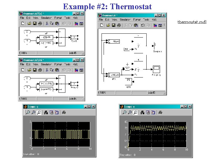
Example #2: Thermostat thermostat. mdl
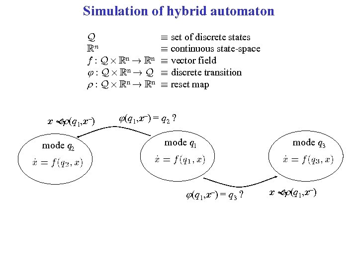
Simulation of hybrid automaton Q Rn f : Q £ Rn ! Rn : Q £ Rn ! Q r : Q £ Rn ! Rn x (q 1, x–) r mode q 2 ´ set of discrete states ´ continuous state-space ´ vector field ´ discrete transition ´ reset map (q 1, x–) = q 2 ? mode q 1 (q 1, x–) = q 3 ? mode q 3 x (q 1, x–) r
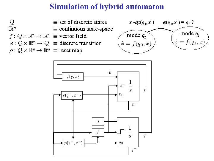
Simulation of hybrid automaton Q Rn f : Q £ Rn ! Rn : Q £ Rn ! Q r : Q £ Rn ! Rn ´ set of discrete states ´ continuous state-space ´ vector field ´ discrete transition ´ reset map x (q 1, x–) r mode q 2 (q 1, x–) = q 2 ? mode q 1
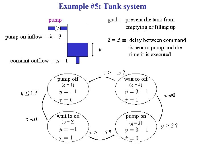
Example #5: Tank system goal ´ prevent the tank from emptying or filling up pump-on inflow ´ l = 3 y constant outflow ´ m = 1 d =. 5 ´ delay between command is sent to pump and the time it is executed t¸ pump off (q = 1) . 5 ? wait to off (q = 4) y· 1? t 0 wait to on pump on (q = 3) (q = 2) t¸ . 5 ? y¸ 2?
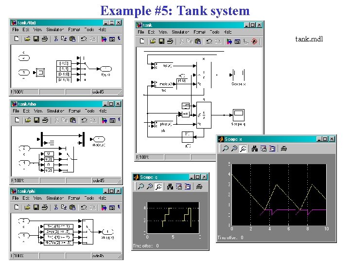
Example #5: Tank system tank. mdl
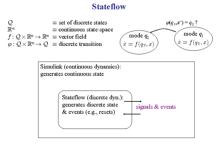
Stateflow Q Rn f : Q £ Rn ! Rn : Q £ Rn ! Q ´ set of discrete states ´ continuous state-space ´ vector field ´ discrete transition (q 1, x–) = q 2 ? mode q 2 Simulink (continuous dynamics): generates continuous state Stateflow (discrete dyn. ): generates discrete state & events (e. g. , resets) signals & events mode q 1
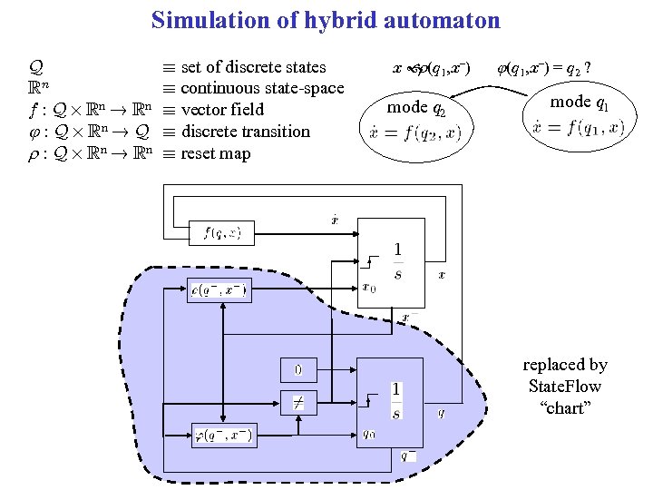
Simulation of hybrid automaton Q Rn f : Q £ Rn ! Rn : Q £ Rn ! Q r : Q £ Rn ! Rn ´ set of discrete states ´ continuous state-space ´ vector field ´ discrete transition ´ reset map x (q 1, x–) r mode q 2 (q 1, x–) = q 2 ? mode q 1 replaced by State. Flow “chart”
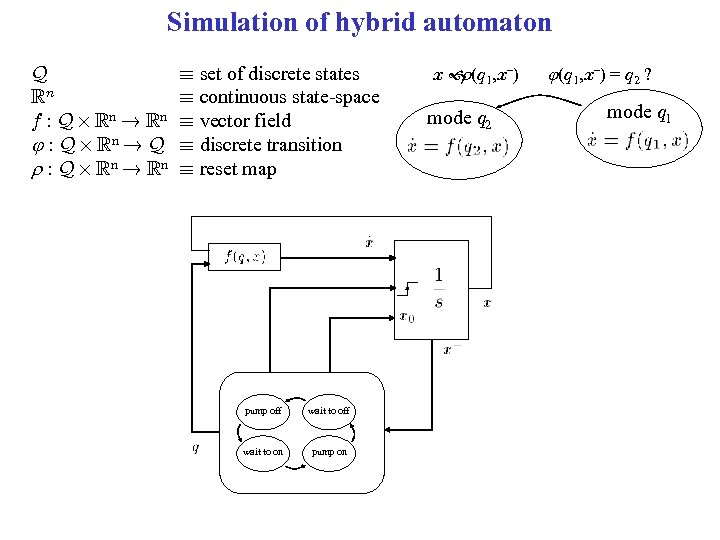
Simulation of hybrid automaton Q Rn f : Q £ Rn ! Rn : Q £ Rn ! Q r : Q £ Rn ! Rn ´ set of discrete states ´ continuous state-space ´ vector field ´ discrete transition ´ reset map pump off wait to on pump on x (q 1, x–) r mode q 2 (q 1, x–) = q 2 ? mode q 1
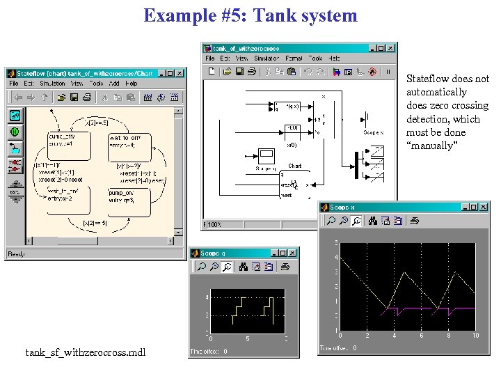
Example #5: Tank system Stateflow does not automatically does zero crossing detection, which must be done “manually” tank_sf_withzerocross. mdl
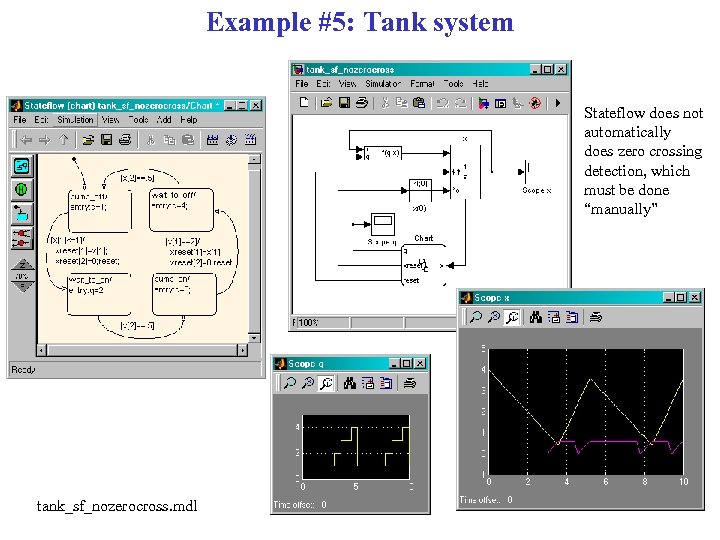
Example #5: Tank system Stateflow does not automatically does zero crossing detection, which must be done “manually” tank_sf_nozerocross. mdl
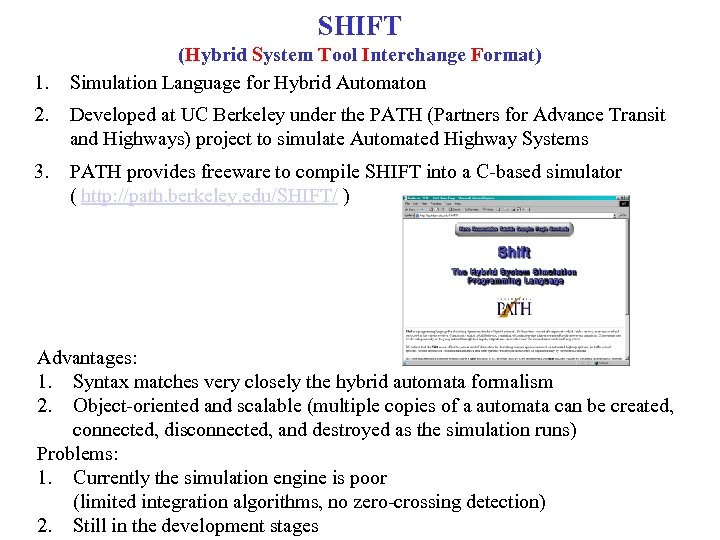
SHIFT 1. (Hybrid System Tool Interchange Format) Simulation Language for Hybrid Automaton 2. Developed at UC Berkeley under the PATH (Partners for Advance Transit and Highways) project to simulate Automated Highway Systems 3. PATH provides freeware to compile SHIFT into a C-based simulator ( http: //path. berkeley. edu/SHIFT/ ) Advantages: 1. Syntax matches very closely the hybrid automata formalism 2. Object-oriented and scalable (multiple copies of a automata can be created, connected, disconnected, and destroyed as the simulation runs) Problems: 1. Currently the simulation engine is poor (limited integration algorithms, no zero-crossing detection) 2. Still in the development stages
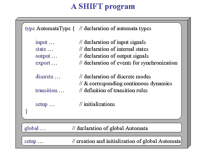
A SHIFT program type Automata. Type { // declaration of automata types input … state … output … export … // declaration of input signals // declaration of internal states // declaration of output signals // declaration of events for synchronization discrete … transition … // declaration of discrete modes // & corresponding continuous dynamics // definition of transition rules setup … // initializations } global … // declaration of global Automata setup … // creation and initialization of global Automata
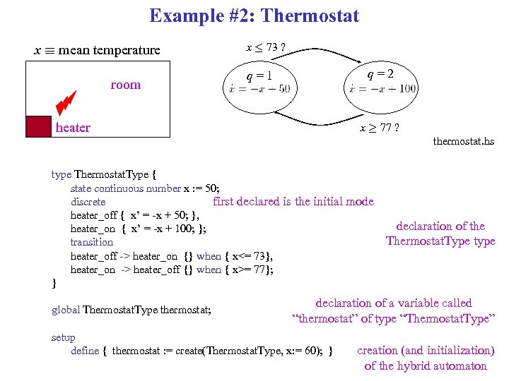
Example #2: Thermostat x ´ mean temperature room x · 73 ? q=2 q=1 heater x ¸ 77 ? thermostat. hs type Thermostat. Type { state continuous number x : = 50; discrete first declared is the initial mode heater_off { x’ = -x + 50; }, heater_on { x’ = -x + 100; }; transition heater_off -> heater_on {} when { x<= 73}, heater_on -> heater_off {} when { x>= 77}; } global Thermostat. Type thermostat; declaration of the Thermostat. Type type declaration of a variable called “thermostat” of type “Thermostat. Type” setup define { thermostat : = create(Thermostat. Type, x: = 60); } creation (and initialization) of the hybrid automaton
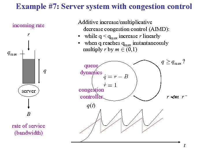
Example #7: Server system with congestion control incoming rate r qmax q server Additive increase/multiplicative decrease congestion control (AIMD): • while q < qmax increase r linearly • when q reaches qmax instantaneously multiply r by m 2 (0, 1) queue dynamics congestion controller q(t) q ¸ qmax ? r r– m B rate of service (bandwidth) t
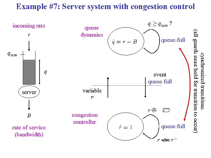
Example #7: Server system with congestion control incoming rate queue-full qmax q server B rate of service (bandwidth) event queue-full variable r congestion controller r> 1 queue-full r r– m synchronized transitions (all guards must hold for transition to occur) r queue dynamics q ¸ qmax ?
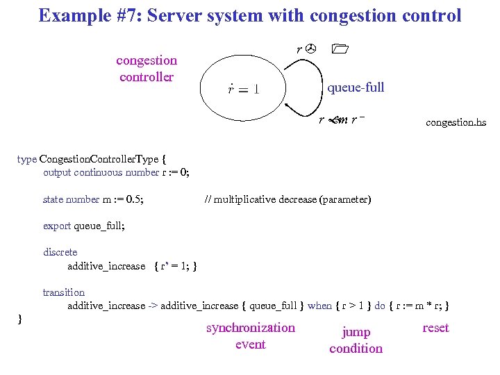
Example #7: Server system with congestion control r> congestion controller 1 queue-full r r– m congestion. hs type Congestion. Controller. Type { output continuous number r : = 0; state number m : = 0. 5; // multiplicative decrease (parameter) export queue_full; discrete additive_increase { r’ = 1; } transition additive_increase -> additive_increase { queue_full } when { r > 1 } do { r : = m * r; } } synchronization event jump condition reset
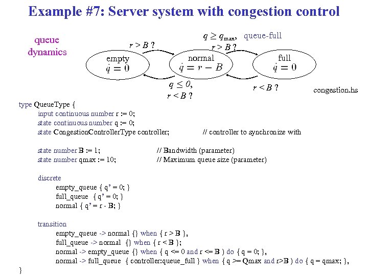
Example #7: Server system with congestion control queue dynamics q ¸ qmax, queue-full r>B? normal full r>B? empty q · 0, r<B? type Queue. Type { input continuous number r : = 0; state continuous number q : = 0; state Congestion. Controller. Type controller; state number B : = 1; state number qmax : = 10; r<B? congestion. hs // controller to synchronize with // Bandwidth (parameter) // Maximum queue size (parameter) discrete empty_queue { q’ = 0; } full_queue { q’ = 0; } normal { q’ = r - B; } transition empty_queue -> normal {} when { r > B }, full_queue -> normal {} when { r < B }; normal -> empty_queue {} when { q <= 0 and r <= B ) do { q = 0; }, normal -> full_queue { controller: queue_full } when { q >= Qmax and r>B ) do { q = qmax; }, }
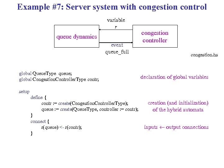
Example #7: Server system with congestion control variable r queue dynamics event queue_full global Queue. Type queue; global Congestion. Controller. Type contr; congestion controller congestion. hs declaration of global variables setup define { contr : = create(Congestion. Controller. Type); queue : = create(Queue. Type, controller : = contr); } connect { r(queue) <- r(contr); } creation (and initialization) of the hybrid automata inputs à output connections
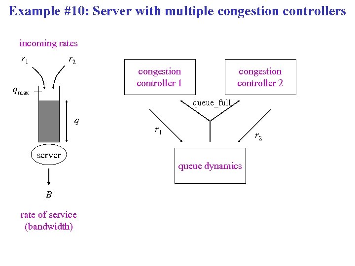
Example #10: Server with multiple congestion controllers incoming rates r 1 r 2 congestion controller 1 qmax congestion controller 2 queue_full q r 1 r 2 server queue dynamics B rate of service (bandwidth)
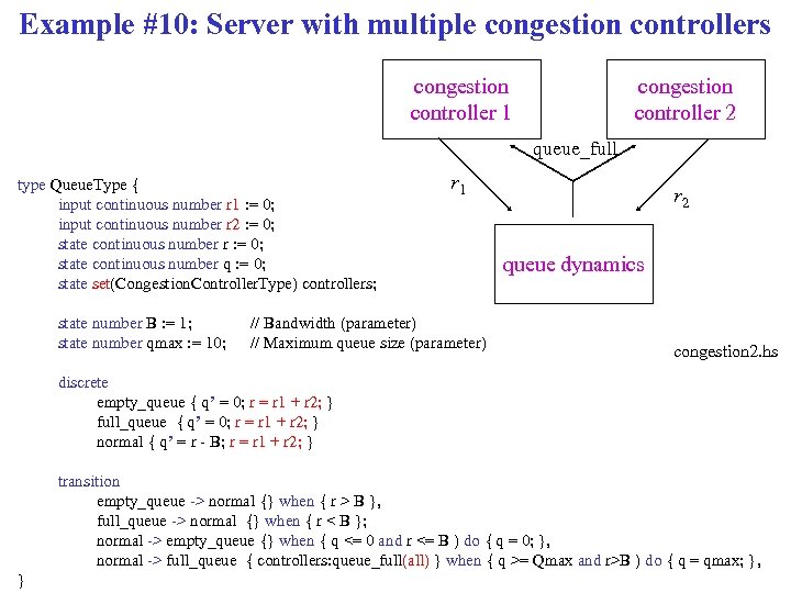
Example #10: Server with multiple congestion controllers congestion controller 1 congestion controller 2 queue_full type Queue. Type { input continuous number r 1 : = 0; input continuous number r 2 : = 0; state continuous number r : = 0; state continuous number q : = 0; state set(Congestion. Controller. Type) controllers; state number B : = 1; state number qmax : = 10; r 1 // Bandwidth (parameter) // Maximum queue size (parameter) r 2 queue dynamics congestion 2. hs discrete empty_queue { q’ = 0; r = r 1 + r 2; } full_queue { q’ = 0; r = r 1 + r 2; } normal { q’ = r - B; r = r 1 + r 2; } transition empty_queue -> normal {} when { r > B }, full_queue -> normal {} when { r < B }; normal -> empty_queue {} when { q <= 0 and r <= B ) do { q = 0; }, normal -> full_queue { controllers: queue_full(all) } when { q >= Qmax and r>B ) do { q = qmax; }, }
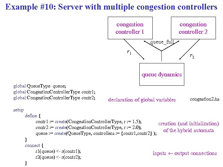
Example #10: Server with multiple congestion controllers congestion controller 1 congestion controller 2 queue_full r 1 r 2 queue dynamics global Queue. Type queue; global Congestion. Controller. Type contr 1; global Congestion. Controller. Type contr 2; declaration of global variables congestion 2. hs setup define { contr 1 : = create(Congestion. Controller. Type, r : = 1. 5); creation (and initialization) contr 2 : = create(Congestion. Controller. Type, r : = 2. 0); of the hybrid automata queue : = create(Queue. Type, controllers : = {contr 1, contr 2} ); } connect { r 1(queue) <- r(contr 1); inputs à output connections r 2(queue) <- r(contr 2); }
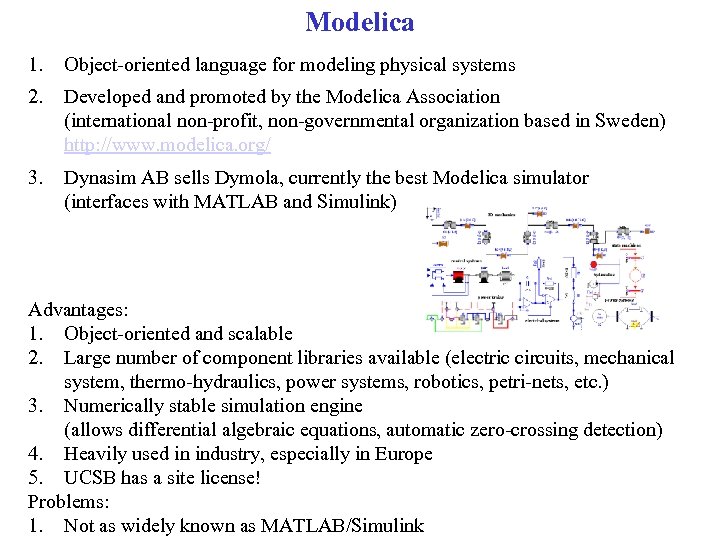
Modelica 1. Object-oriented language for modeling physical systems 2. Developed and promoted by the Modelica Association (international non-profit, non-governmental organization based in Sweden) http: //www. modelica. org/ 3. Dynasim AB sells Dymola, currently the best Modelica simulator (interfaces with MATLAB and Simulink) Advantages: 1. Object-oriented and scalable 2. Large number of component libraries available (electric circuits, mechanical system, thermo-hydraulics, power systems, robotics, petri-nets, etc. ) 3. Numerically stable simulation engine (allows differential algebraic equations, automatic zero-crossing detection) 4. Heavily used in industry, especially in Europe 5. UCSB has a site license! Problems: 1. Not as widely known as MATLAB/Simulink
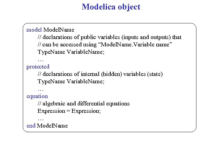
Modelica object model Model. Name // declarations of public variables (inputs and outputs) that // can be accessed using “Model. Name. Variable name” Type. Name Variable. Name; … protected // declarations of internal (hidden) variables (state) Type. Name Variable. Name; … equation // algebraic and differential equations Expression = Expression; … end Model. Name
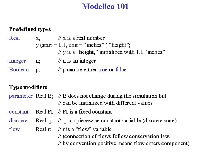
Modelica 101 Predefined types Real x, // x is a real number y (start = 1. 1, unit = “inches” ) “height”; // y is a “height, ” initialized with 1. 1 “inches” Integer n; // n is an integer Boolean p; // p can be either true or false Type modifiers parameter Real B; // B does not change during the simulation but // can be initialized with different values constant Real PI; // PI is a fixed constant discrete Real q; // q is a piecewise constant variable (discrete state) flow Real r; // r is a “flow” variable // (connection of flows follow conservation law, // by convention positive means flow enters component)
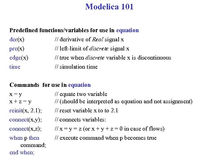
Modelica 101 Predefined functions/variables for use in equation der(x) // derivative of Real signal x pre(x) // left-limit of discrete signal x edge(x) // true when discrete variable x is discontinuous time // simulation time Commands for use in equation x=y // equate two variable x+z=y // (should be interpreted as equation and not assignment) reinit(x, 2. 1); // reset variable x to to 2. 1 connect(x, y); // connects variables: connect(x, z); // x = y = z (or x + y + z = 0 in case of flows) when p then // execute command when p becomes true command; end when;
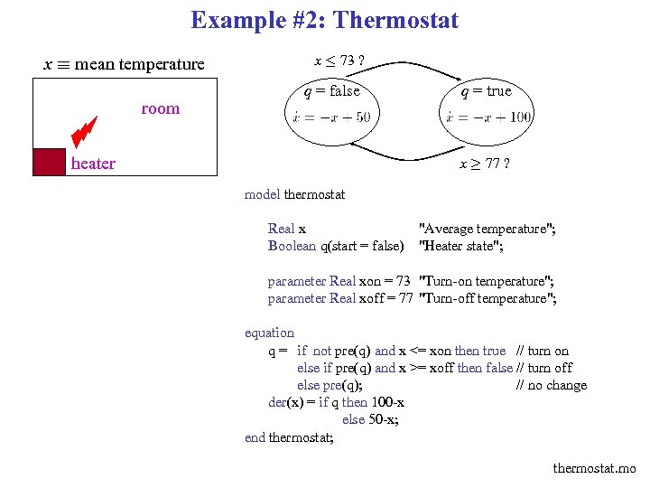
Example #2: Thermostat x ´ mean temperature room x · 73 ? q = false heater q = true x ¸ 77 ? model thermostat Real x "Average temperature"; Boolean q(start = false) "Heater state"; parameter Real xon = 73 "Turn-on temperature"; parameter Real xoff = 77 "Turn-off temperature"; equation q = if not pre(q) and x <= xon then true // turn on else if pre(q) and x >= xoff then false // turn off else pre(q); // no change der(x) = if q then 100 -x else 50 -x; end thermostat; thermostat. mo
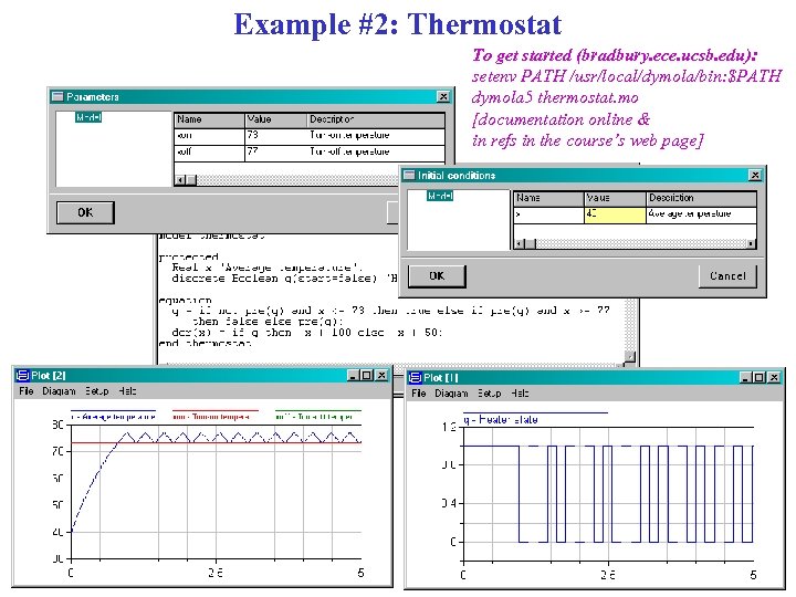
Example #2: Thermostat To get started (bradbury. ece. ucsb. edu): setenv PATH /usr/local/dymola/bin: $PATH dymola 5 thermostat. mo [documentation online & in refs in the course’s web page]
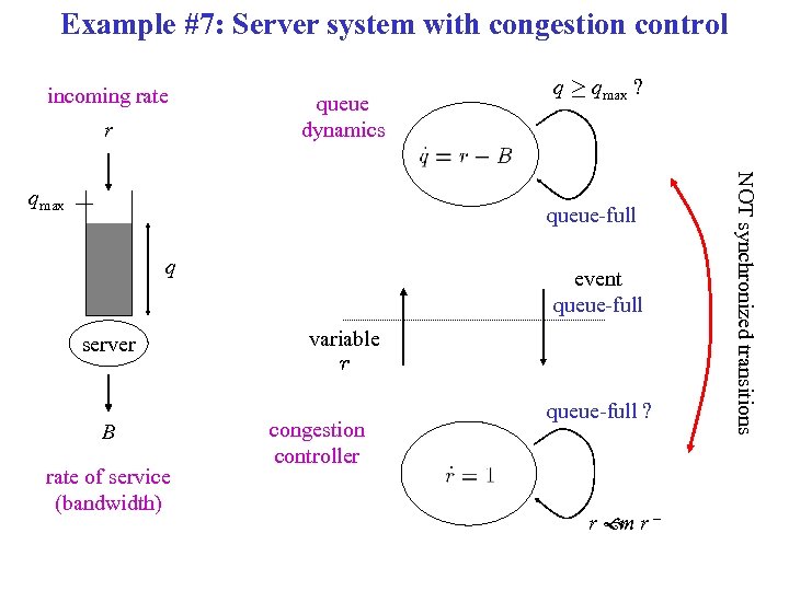
Example #7: Server system with congestion control incoming rate r queue dynamics queue-full q server B rate of service (bandwidth) event queue-full variable r congestion controller queue-full ? r r– m NOT synchronized transitions qmax q ¸ qmax ?
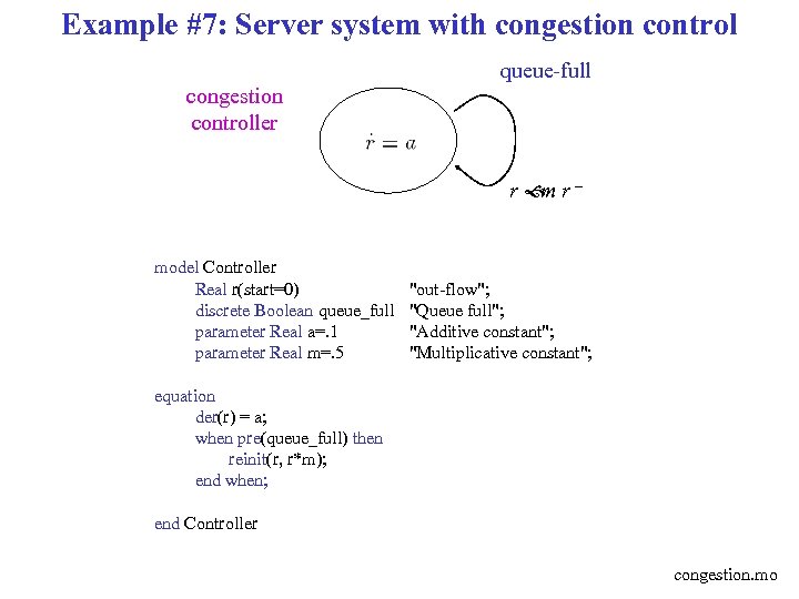
Example #7: Server system with congestion control queue-full congestion controller r r– m model Controller Real r(start=0) discrete Boolean queue_full parameter Real a=. 1 parameter Real m=. 5 "out-flow"; "Queue full"; "Additive constant"; "Multiplicative constant"; equation der(r) = a; when pre(queue_full) then reinit(r, r*m); end when; end Controller congestion. mo
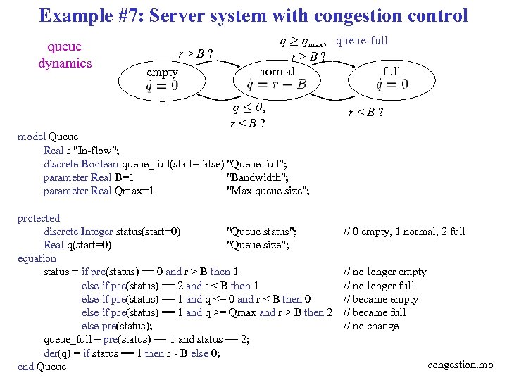
Example #7: Server system with congestion control queue dynamics r>B? empty q ¸ qmax, queue-full r>B? normal full q · 0, r<B? model Queue Real r "In-flow"; discrete Boolean queue_full(start=false) "Queue full"; parameter Real B=1 "Bandwidth"; parameter Real Qmax=1 "Max queue size"; protected discrete Integer status(start=0) "Queue status"; Real q(start=0) "Queue size"; equation status = if pre(status) == 0 and r > B then 1 else if pre(status) == 2 and r < B then 1 else if pre(status) == 1 and q <= 0 and r < B then 0 else if pre(status) == 1 and q >= Qmax and r > B then 2 else pre(status); queue_full = pre(status) == 1 and status == 2; der(q) = if status == 1 then r - B else 0; end Queue // 0 empty, 1 normal, 2 full // no longer empty // no longer full // became empty // became full // no change congestion. mo
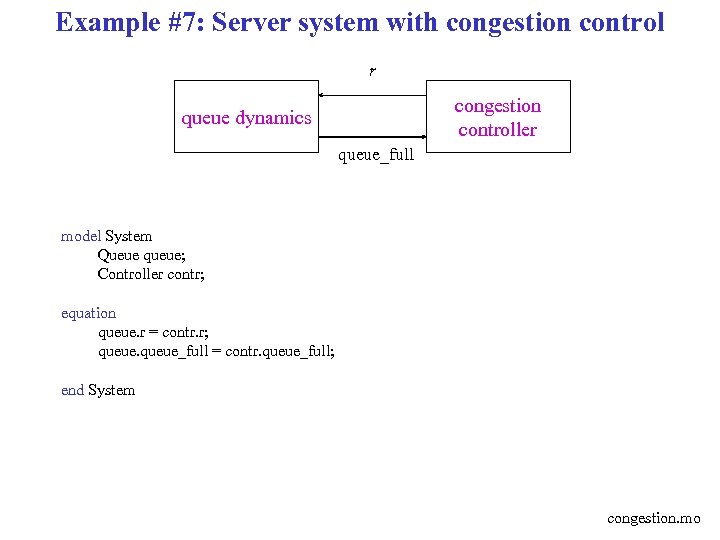
Example #7: Server system with congestion control r congestion controller queue dynamics queue_full model System Queue queue; Controller contr; equation queue. r = contr. r; queue_full = contr. queue_full; end System congestion. mo
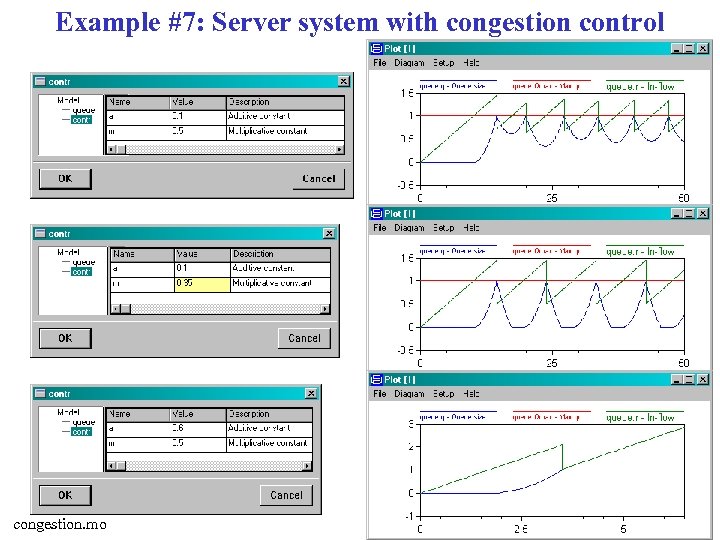
Example #7: Server system with congestion control congestion. mo
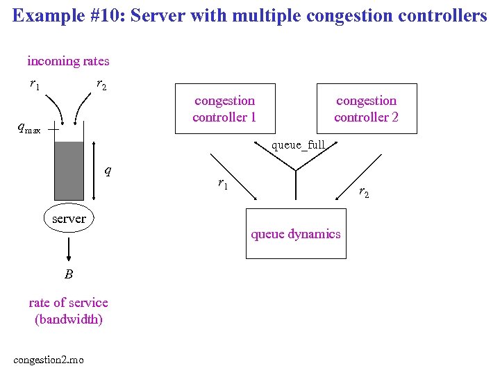
Example #10: Server with multiple congestion controllers incoming rates r 1 r 2 congestion controller 1 qmax congestion controller 2 queue_full q r 1 r 2 server queue dynamics B rate of service (bandwidth) congestion 2. mo
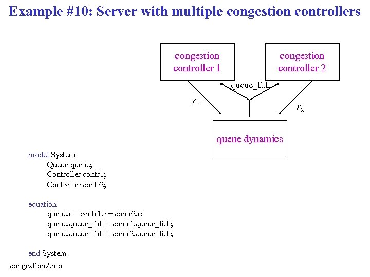
Example #10: Server with multiple congestion controllers congestion controller 1 congestion controller 2 queue_full r 1 r 2 queue dynamics model System Queue queue; Controller contr 1; Controller contr 2; equation queue. r = contr 1. r + contr 2. r; queue_full = contr 1. queue_full; queue_full = contr 2. queue_full; end System congestion 2. mo
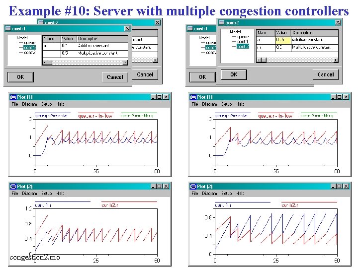
Example #10: Server with multiple congestion controllers congestion 2. mo
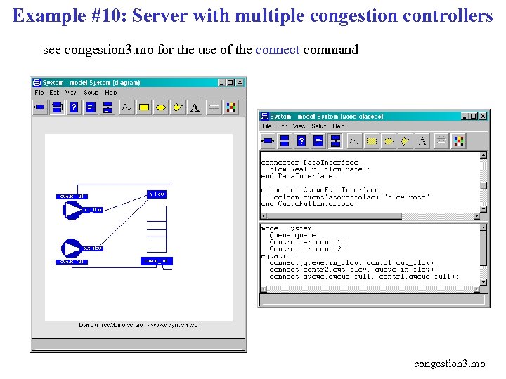
Example #10: Server with multiple congestion controllers see congestion 3. mo for the use of the connect command congestion 3. mo
Interfacing Dymola & MATLAB/Simulink Sharing data • Each time you simulate a Dymola model, a file “xxxx. mat” is created with all the data. You can get this data into MATLAB with load xxxx. mat Using Dymola models in Simulink • Add dymola to the MATLAB path: path('/usr/local/dymola/mfiles', path) path('/usr/local/dymola/mfiles/traj', path) • The Simulink block /usr/local/dymola/mfiles/Dymola. Block. Master. mdl can be used to insert a Dymola system into a Simulink diagram Not sure if its working?
Next class… Properties of hybrid systems • Safety (reachability) • Liveness • Asymptotic properties (stability)
f29230dac59df7a6c5be4bc0c05c681c.ppt