How to use propensity scores in the analysis

How to use propensity scores in the analysis of nonrandomized designs Patrick G. Arbogast Department of Biostatistics Vanderbilt University Medical Center 2007 Jan 05 GCRC Research-Skills Workshop 1

2007 Jan 05 GCRC Research-Skills Workshop 2

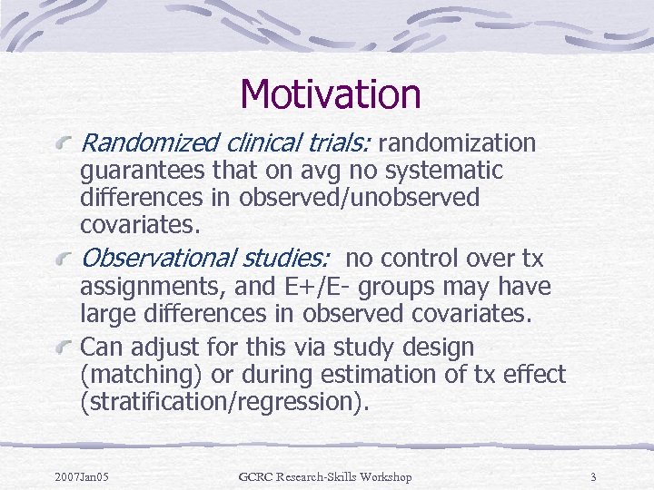Motivation Randomized clinical trials: randomization guarantees that on avg no systematic differences in observed/unobserved covariates. Observational studies: no control over tx assignments, and E+/E- groups may have large differences in observed covariates. Can adjust for this via study design (matching) or during estimation of tx effect (stratification/regression). 2007 Jan 05 GCRC Research-Skills Workshop 3

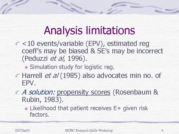Analysis limitations <10 events/variable (EPV), estimated reg coeff’s may be biased & SE’s may be incorrect (Peduzzi et al, 1996). Simulation study for logistic reg. Harrell et al (1985) also advocates min no. of EPV. A solution: propensity scores (Rosenbaum & Rubin, 1983). Likelihood that patient receives E+ given risk factors. 2007 Jan 05 GCRC Research-Skills Workshop 4

Intuition Covariate is confounder only if its distribution in E+/E- differ. Consider 1 -factor matching: low-dose aspirin & mortality. Age, a strong confounder, can be controlled by matching. Can extend to many risk factors, but becomes cumbersome. Propensity scores provide a summary measure to control for multiple confounders simultaneously. 2007 Jan 05 GCRC Research-Skills Workshop 5

Propensity score estimation Identify potential confounders. Current conventional wisdom: if uncertain whether covariate is confounder, include it. Model E+ (typically dichotomous) as function of covariates using entire cohort. E+ is outcome for propensity score estimation. Do not include D+. Logistic reg typically used. Propensity score = estimated Pr(E+|covariates). 2007 Jan 05 GCRC Research-Skills Workshop 6

Counterintuitive? Natural question: why estimate probability that a patient receives E+ since we already know exposure status? Answer: adjusting observed E+ with probability of E+ (“propensity”) creates a “quasi-randomized” experiment. For E+ & E- patients with same propensity score, can imagine they were “randomly” assigned to each group. Subjects in E+/E- groups with equal (or nearly equal) propensity scores tend to have similar distribution in covariates used to estimate propensity. 2007 Jan 05 GCRC Research-Skills Workshop 7

Balancing score For given propensity score, one gets unbiased estimates of avg E+ effect. Can include large no. of covariates for propensity score estimation. In fact, original paper applied propensity score methodology to observational study comparing CABG to medical tx, adjusting for 74 covariates in propensity model. 2007 Jan 05 GCRC Research-Skills Workshop 8

Applications Matching. Regression adjustment/stratification. Weighting. 2007 Jan 05 GCRC Research-Skills Workshop 9

Propensity score matching Match on single summary measure. Useful for studies with limited no. of E+ patients and a larger (usually much larger) no. of E- patients & need to collect add’l measures (eg, blood samples). 2007 Jan 05 GCRC Research-Skills Workshop 10

Matching techniques Nearest available matching on estimated propensity score. Select E+ subject. Find E- subjecdt w/ closest propensity score. Repeat until all E+ subjects matched. Easiest in terms of computational considerations. Others: Mahalanobis metric matching. Nearest available Mahalanobis metric matching w/ propensity score-based calipers. 2007 Jan 05 GCRC Research-Skills Workshop 11

Illustrative example Consider an HIV database: E+: patients receiving a new antiretroviral drug (N=500). E-: patients not receiving the drug (N=10, 000). D+: mortality. Need to manually measure CD 4. May be potential confounding by other HIV drugs as well as 10 prognostic factors, which are identified & stored in the database. 2007 Jan 05 GCRC Research-Skills Workshop 12

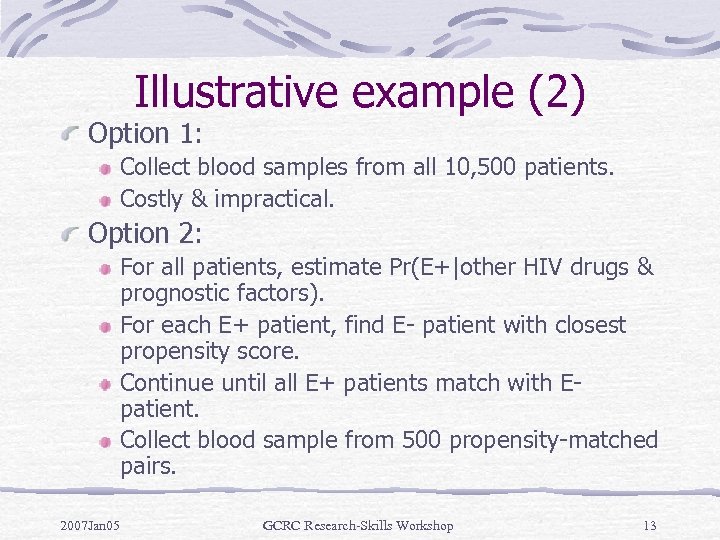Illustrative example (2) Option 1: Collect blood samples from all 10, 500 patients. Costly & impractical. Option 2: For all patients, estimate Pr(E+|other HIV drugs & prognostic factors). For each E+ patient, find E- patient with closest propensity score. Continue until all E+ patients match with Epatient. Collect blood sample from 500 propensity-matched pairs. 2007 Jan 05 GCRC Research-Skills Workshop 13

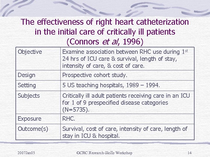The effectiveness of right heart catheterization in the initial care of critically ill patients (Connors et al, 1996) Objective Examine association between RHC use during 1 st 24 hrs of ICU care & survival, length of stay, intensity of care, & cost of care. Design Prospective cohort study. Setting 5 US teaching hospitals, 1989 – 1994. Subjects Critically ill adult patients receiving care in an ICU for 1 of 9 prespecified disease categories (N=5735). Exposure RHC. Outcome(s) Survival, cost of care, intensity of care, length of stay in ICU & hospital. 2007 Jan 05 GCRC Research-Skills Workshop 14

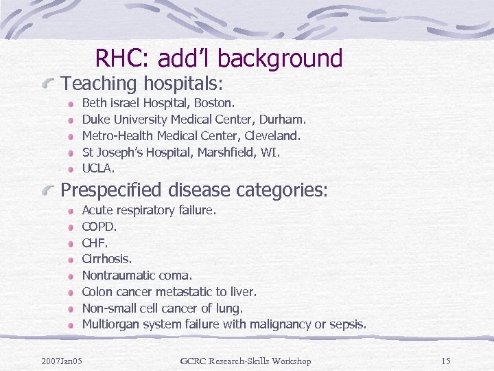RHC: add’l background Teaching hospitals: Beth israel Hospital, Boston. Duke University Medical Center, Durham. Metro-Health Medical Center, Cleveland. St Joseph’s Hospital, Marshfield, WI. UCLA. Prespecified disease categories: Acute respiratory failure. COPD. CHF. Cirrhosis. Nontraumatic coma. Colon cancer metastatic to liver. Non-small cell cancer of lung. Multiorgan system failure with malignancy or sepsis. 2007 Jan 05 GCRC Research-Skills Workshop 15

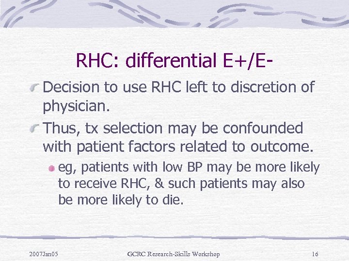RHC: differential E+/EDecision to use RHC left to discretion of physician. Thus, tx selection may be confounded with patient factors related to outcome. eg, patients with low BP may be more likely to receive RHC, & such patients may also be more likely to die. 2007 Jan 05 GCRC Research-Skills Workshop 16

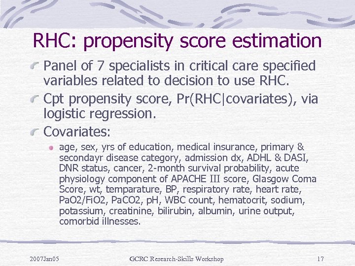RHC: propensity score estimation Panel of 7 specialists in critical care specified variables related to decision to use RHC. Cpt propensity score, Pr(RHC|covariates), via logistic regression. Covariates: age, sex, yrs of education, medical insurance, primary & secondayr disease category, admission dx, ADHL & DASI, DNR status, cancer, 2 -month survival probability, acute physiology component of APACHE III score, Glasgow Coma Score, wt, temparature, BP, respiratory rate, heart rate, Pa. O 2/Fi. O 2, Pa. CO 2, p. H, WBC count, hematocrit, sodium, potassium, creatinine, bilirubin, albumin, urine output, comorbid illnesses. 2007 Jan 05 GCRC Research-Skills Workshop 17

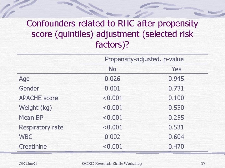
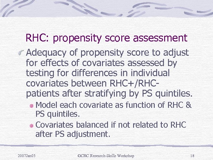RHC: propensity score assessment Adequacy of propensity score to adjust for effects of covariates assessed by testing for differences in individual covariates between RHC+/RHCpatients after stratifying by PS quintiles. Model each covariate as function of RHC & PS quintiles. Covariates balanced if not related to RHC after PS adjustment. 2007 Jan 05 GCRC Research-Skills Workshop 18

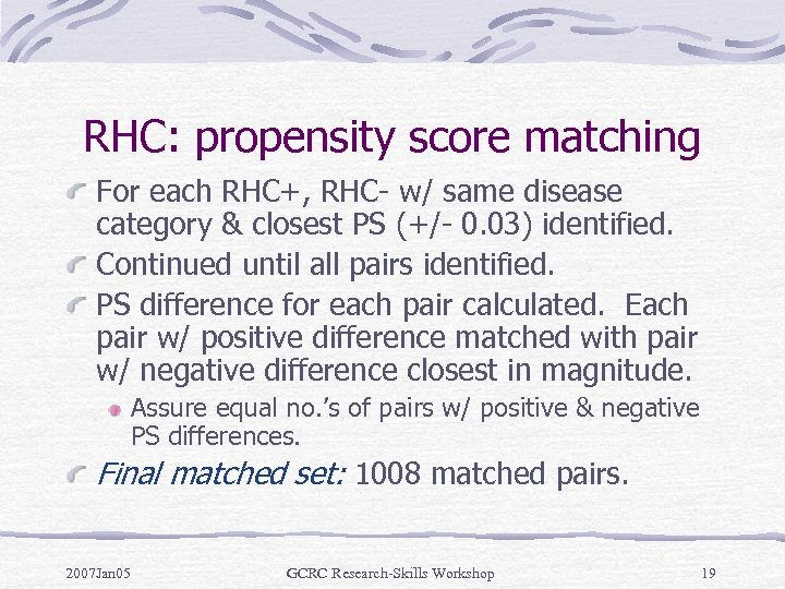RHC: propensity score matching For each RHC+, RHC- w/ same disease category & closest PS (+/- 0. 03) identified. Continued until all pairs identified. PS difference for each pair calculated. Each pair w/ positive difference matched with pair w/ negative difference closest in magnitude. Assure equal no. ’s of pairs w/ positive & negative PS differences. Final matched set: 1008 matched pairs. 2007 Jan 05 GCRC Research-Skills Workshop 19

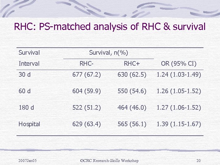RHC: PS-matched analysis of RHC & survival Survival Interval Survival, n(%) RHC- RHC+ OR (95% CI) 30 d 677 (67. 2) 630 (62. 5) 1. 24 (1. 03 -1. 49) 60 d 604 (59. 9) 550 (54. 6) 1. 26 (1. 05 -1. 52) 180 d 522 (51. 2) 464 (46. 0) 1. 27 (1. 06 -1. 52) Hospital 629 (63. 4) 565 (56. 1) 1. 39 (1. 15 -1. 67) 2007 Jan 05 GCRC Research-Skills Workshop 20

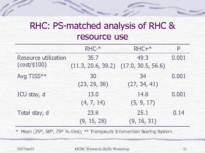RHC: PS-matched analysis of RHC & resource use RHC-* RHC+* P Resource utilization 35. 7 49. 3 (cost/$100) (11. 3, 20. 6, 39. 2) (17. 0, 30. 5, 56. 6) 0. 001 Avg TISS** 30 (23, 29, 38) 34 (27, 34, 41) 0. 001 ICU stay, d 13. 0 (4, 7, 14) 14. 8 (5, 9, 17) 0. 001 Total stay, d 23. 8 (9, 15, 28) 25. 1 (9, 16, 31) 0. 14 * Mean (25 th, 50 th, 75 th %-tiles); ** Therapeutic Intervention Scoring System. 2007 Jan 05 GCRC Research-Skills Workshop 21

Regression adjustment/stratification Stratification on PS alone can balance distributions of covariates in E+/E- groups w/o exponential increase in no. of strata. Rosenbaum & Rubin (1983) showed that perfect stratification based on PS will produce strata where avg tx effect w/i strata is unbiased estimate of true tx effect. 2007 Jan 05 GCRC Research-Skills Workshop 22

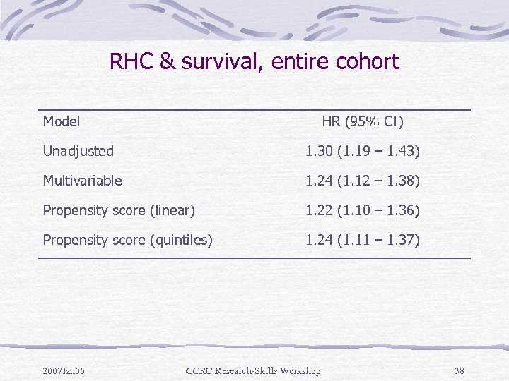
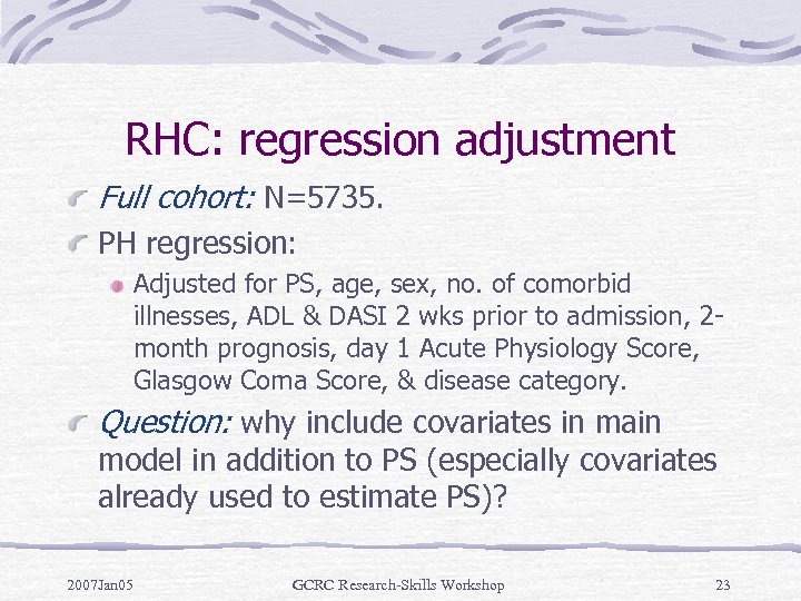RHC: regression adjustment Full cohort: N=5735. PH regression: Adjusted for PS, age, sex, no. of comorbid illnesses, ADL & DASI 2 wks prior to admission, 2 month prognosis, day 1 Acute Physiology Score, Glasgow Coma Score, & disease category. Question: why include covariates in main model in addition to PS (especially covariates already used to estimate PS)? 2007 Jan 05 GCRC Research-Skills Workshop 23

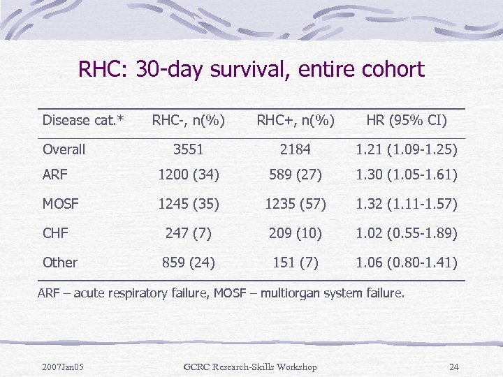RHC: 30 -day survival, entire cohort Disease cat. * RHC-, n(%) RHC+, n(%) HR (95% CI) 3551 2184 1. 21 (1. 09 -1. 25) ARF 1200 (34) 589 (27) 1. 30 (1. 05 -1. 61) MOSF 1245 (35) 1235 (57) 1. 32 (1. 11 -1. 57) CHF 247 (7) 209 (10) 1. 02 (0. 55 -1. 89) Other 859 (24) 151 (7) 1. 06 (0. 80 -1. 41) Overall ARF – acute respiratory failure, MOSF – multiorgan system failure. 2007 Jan 05 GCRC Research-Skills Workshop 24

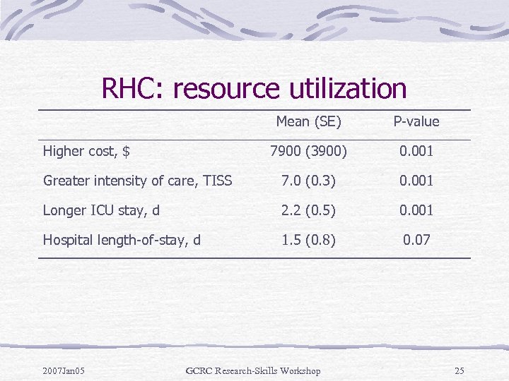RHC: resource utilization Mean (SE) P-value 7900 (3900) 0. 001 Greater intensity of care, TISS 7. 0 (0. 3) 0. 001 Longer ICU stay, d 2. 2 (0. 5) 0. 001 Hospital length-of-stay, d 1. 5 (0. 8) 0. 07 Higher cost, $ 2007 Jan 05 GCRC Research-Skills Workshop 25

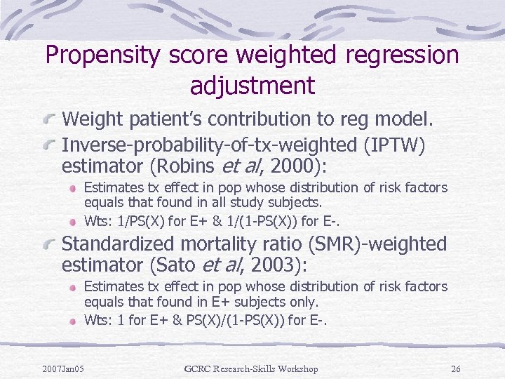Propensity score weighted regression adjustment Weight patient’s contribution to reg model. Inverse-probability-of-tx-weighted (IPTW) estimator (Robins et al, 2000): Estimates tx effect in pop whose distribution of risk factors equals that found in all study subjects. Wts: 1/PS(X) for E+ & 1/(1 -PS(X)) for E-. Standardized mortality ratio (SMR)-weighted estimator (Sato et al, 2003): Estimates tx effect in pop whose distribution of risk factors equals that found in E+ subjects only. Wts: 1 for E+ & PS(X)/(1 -PS(X)) for E-. 2007 Jan 05 GCRC Research-Skills Workshop 26

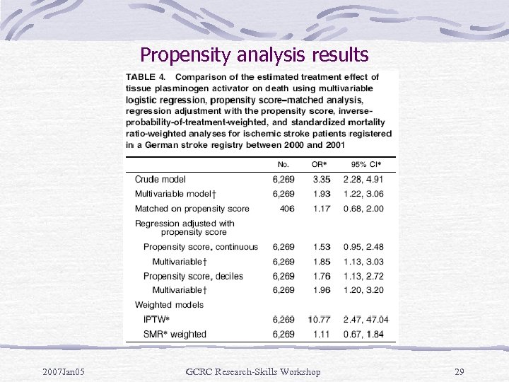
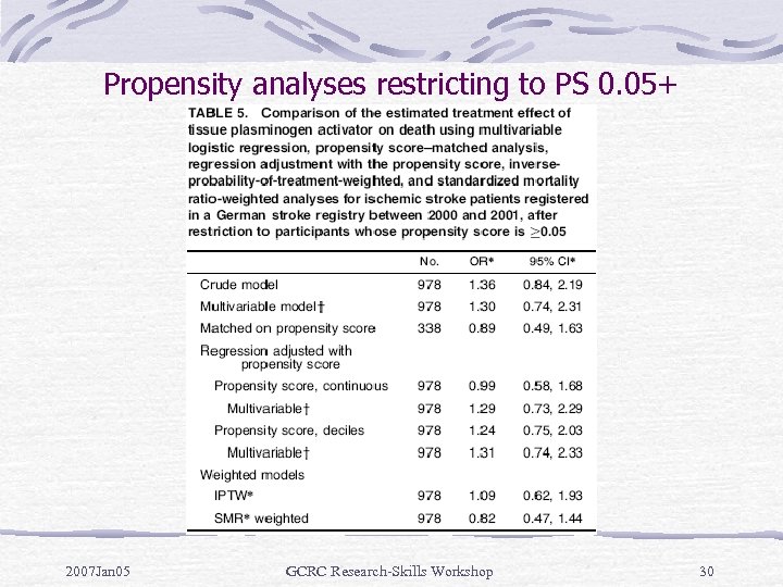
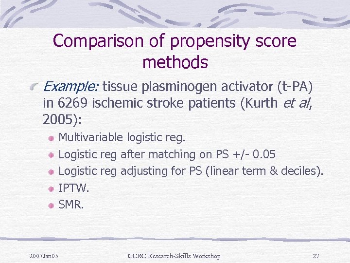Comparison of propensity score methods Example: tissue plasminogen activator (t-PA) in 6269 ischemic stroke patients (Kurth et al, 2005): Multivariable logistic reg. Logistic reg after matching on PS +/- 0. 05 Logistic reg adjusting for PS (linear term & deciles). IPTW. SMR. 2007 Jan 05 GCRC Research-Skills Workshop 27

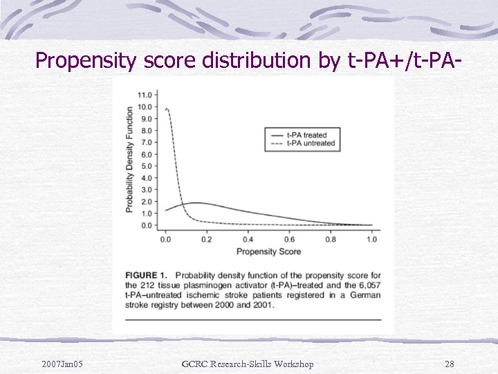Propensity score distribution by t-PA+/t-PA- 2007 Jan 05 GCRC Research-Skills Workshop 28

Propensity analysis results 2007 Jan 05 GCRC Research-Skills Workshop 29

Propensity analyses restricting to PS 0. 05+ 2007 Jan 05 GCRC Research-Skills Workshop 30

Propensity score vs other methods Matching on individual factors: Too cumbersome (eg, matching on 10 factors, each having 4 categories, resulting in ~1, 000 combinations of patient characteristics). Stratified analyses: same problem. Regression (Cepeda et al, 2003): <7 events/confounder – PS less biased, more robust, & more precise. 8+ events/confounder – multiple reg preferable: Bias from multiple reg goes away, but still present for PS analysis (eg, ~25 -30% bias when OR=2. 0). Coverage probability (% of 95% CI’s containing true OR) decreases for PS analysis. 2007 Jan 05 GCRC Research-Skills Workshop 31

Benefits: Useful when adjusting for large no. of risk factors & small no. of EPV. Useful for matched designs (saving time & money). Can be applied to exposure with 3+ levels (Rosenbaum, 2002). 2007 Jan 05 GCRC Research-Skills Workshop 32

Limitations Can only adjust for observed covariates. Propensity score methods work better in larger samples to attain distributional balance of observed covariates. In small studies, imbalances may be unavoidable. Including irrelevant covariates in propensity model may reduce efficiency. Bias may occur. Non-uniform tx effect. 2007 Jan 05 GCRC Research-Skills Workshop 33

Sample propensity analysis: RHC E+: RHC use. swang 1 (0=RHC-, 1=RHC+) D+: time-to-death, min(obs time, 30 d). Events after 30 d censored. RHC could not have a long-term effect. Such ill patients more affected by later tx decisions. t 3 d 30, censor var=censor N=5735 patients, N=1918 deaths w/i 30 d. 38. 0% RHC+ & 30. 6% RHC- died w/i 30 d. 2007 Jan 05 GCRC Research-Skills Workshop 34

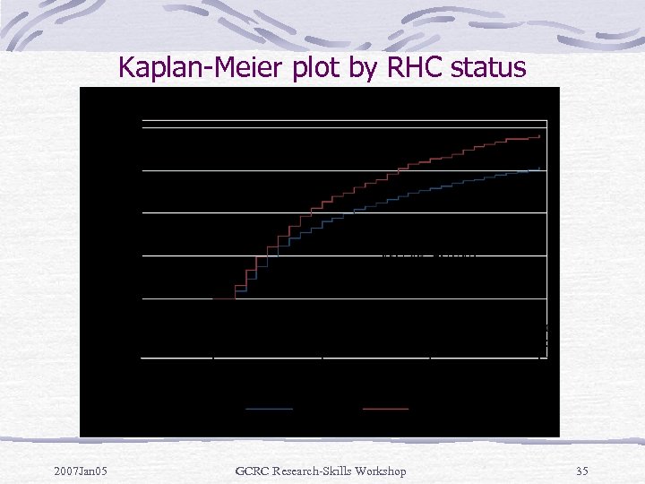Kaplan-Meier plot by RHC status 2007 Jan 05 GCRC Research-Skills Workshop 35

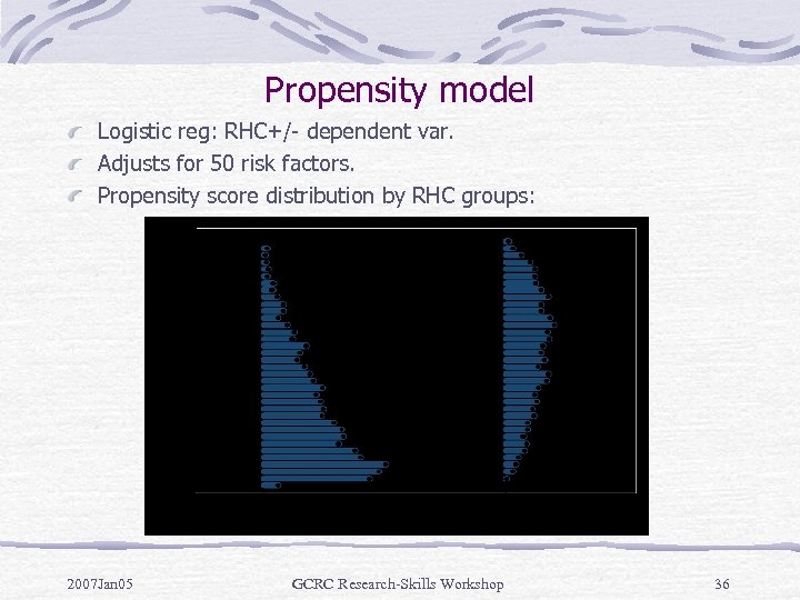Propensity model Logistic reg: RHC+/- dependent var. Adjusts for 50 risk factors. Propensity score distribution by RHC groups: 2007 Jan 05 GCRC Research-Skills Workshop 36

Confounders related to RHC after propensity score (quintiles) adjustment (selected risk factors)? Propensity-adjusted, p-value No Yes Age 0. 026 0. 945 Gender 0. 001 0. 731 APACHE score <0. 001 0. 100 Weight (kg) <0. 001 0. 530 Mean BP <0. 001 0. 255 Respiratory rate <0. 001 0. 531 0. 002 0. 604 <0. 001 0. 470 WBC Creatinine 2007 Jan 05 GCRC Research-Skills Workshop 37

RHC & survival, entire cohort Model HR (95% CI) Unadjusted 1. 30 (1. 19 – 1. 43) Multivariable 1. 24 (1. 12 – 1. 38) Propensity score (linear) 1. 22 (1. 10 – 1. 36) Propensity score (quintiles) 1. 24 (1. 11 – 1. 37) 2007 Jan 05 GCRC Research-Skills Workshop 38

References Cepeda MS, Boston R, Farrar JT, Strom BL. Comparison of logistic regression versus propensity score when the number of events is low and there are multiple confounders. Am J Epidemiol 2003; 158: 280287. Connors Jr AF, Speroff T, Dawson NV, et al. The effectiveness of right heart catheterization in the initial care of critically ill patients. JAMA 1996; 276: 889 -897. D’Agostino Jr, RB. Tutorial in biostatistics: propensity score methods for bias reduction in the comparison of a treatment to a non-randomized control group. Stat Med 1998; 17: 2265 -2281. Gum PA, Thamilarasan M, Watanabe J, Blackstone EH, Lauer MS. Aspirin use and all-cause mortality among patients being evaluated for known or suspected coronary artery disease. JAMA 2001; 286: 11871194. Harrell FE, Lee KL, Matchar DB, Reichart TA. Regression models for prognostic prediction: advantages, problems, and suggested solutions. Cancer Treatment Reports 1985: 69: 1071 -1077. Kurth T, Walker AM, Glynn RJ, Chan KA, Gaziano JM, Berger K, Robins JM. Results of multivariable logistic regrssion, propensity matching, propensity adjustment, and propensity-based weighting under conditions of nonuniform effect. Am J Epidemiol 2006; 163: 262 -270. Peduzzi P, Concato J, Kemper E, Holford TR, Feinstein AR. A simulation study of the number of events per variable in logistic regression analysis. J Clin Epidemiol 1996; 49: 1373 -1379. Robins JM, Hernan MA, Brumback B. Marginal structural models and causal inference in epidemiology. Epidemiology 2000; 11: 550 -560. Rosenbaum PR. Observational Studies. New York, NY: Springer-Verlag, 2002. Rosenbaum PR, Rubin DB. The central rol of the propensity score in observational studies for causal effects. Biometrika 1983; 70: 41 -55. Rubin DB. Estimating causal effects from large data sets using propensity scores. Annals of Internal Medicine 1997; 127: 757 -763. Sato T, Matsuyama Y. Marginal structural models as a tool for standardization. Epidemiology 2003; 14: 680 -686. 2007 Jan 05 GCRC Research-Skills Workshop 39