9e452fa124f7590fe108edeac81303be.ppt
- Количество слайдов: 16

How to measure potential bank systemic risk and identify contributing banks? Presentation for The determinants of domestic and cross border bank contagion risk in South East Asia Carlos BAUTISTA, Philippe ROUS, Amine TARAZI European Commission ASIA-LINK project : Safety and Soundness of the Financial System, Université de Limoges (www. upd. edu/~cba/asialink)

BACKGROUND AND RESEARCH MOTIVATION Asian financial crisis and role played by banking institutions (at the forefront) Cross border banking and regulation and supervision (Holh et alii (2005)) • Post Crisis literature insists on contagion effects (See for example, Kaminsky and Reinhart (2000)). • An area of research on contagion that has not been fully explored is concerned with systemic risk at the banking sector level in Asia. • There are only a few studies on bank domestic contagion for the Asian region (See for example, Bystrom, (2004)). What about Cross border contagion? 2

AIM OF THE PAPER Build a framework based on stock prices to measure bank potential contagion risk after the Asian Crisis episode and to specifically assess their determinants at the domestic and cross border levels 2 questions : • Are there country differences in potential bank contagion risk in South East Asia and spillover effects (both domestic and cross border potential risk) ? • Can we determine the profile of banks that contribute the most to systemic risk (capture the main determinants of individual bank exposure) ? 3

PRESENTATION 1. Method and Model Specification What measure of contagion? Why use alternative specifications and why test for stability and robustness? Stepwise multivariate probit model/fixed effect panel data model to identify bank contagion specific factors 2. Data Individuals : 125 listed banks (8 countries in South Est Asia) Time Period : 2000 – 2005 3. Results 4. Conclusion 4
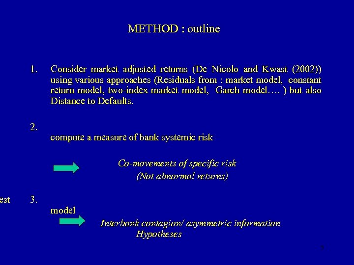
est METHOD : outline 1. 2. Consider market adjusted returns (De Nicolo and Kwast (2002)) using various approaches (Residuals from : market model, constant return model, two-index market model, Garch model…. ) but also Distance to Defaults. compute a measure of bank systemic risk Co-movements of specific risk (Not abnormal returns) 3. model Interbank contagion/ asymmetric information Hypotheses 5
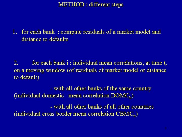
METHOD : different steps 1. for each bank : compute residuals of a market model and distance to defaults 2. for each bank i : individual mean correlations, at time t, on a moving window (of residuals of market model or distance to default) - with all other banks of the same country (individual domestic mean correlation DOMCit) - with all other banks of all other countries (individual cross border mean correlation CBMCit) 6

3. For each country P, we compute the cross section average, at time t, - of the individual domestic mean correlations (DOMCPt) - of the individual cross border mean correlations (CBMCPt) and test for their significance Country cross section averages measure, at time t, the magnitude of potential systemic risk in this country 4. We assess the contribution of each bank i(P) to its country P domestic / cross border average correlation level by estimating the two models : DOMCi(P) t = ai + li DOMCP t + eit CBMCi(P) t = ai’ + li’ CBMCP t + eit Sensitivity in terms of co-movements

5. we define two binary variables : DP_DOMi = 1 if li > 1 significantly and 0 otherwise DP_CBi = 1 if li’ > 1 significantly and 0 otherwise 6. we try to explain the probability of DP_DOMi = 1 (resp. DP_CBi = 1) by estimating a probit model : where Chi and Mki are size / bank structure accounting regressors and market based risk indicators relative to bank i ; F(. ) is the cumulative of the normal distribution
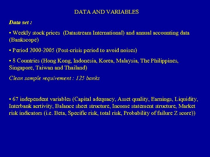
DATA AND VARIABLES Data set : • Weekly stock prices (Datastream International) and annual accounting data (Bankscope) • Period 2000 -2005 (Post-crisis period to avoid noises) • 8 Countries (Hong Kong, Indonesia, Korea, Malaysia, The Philippines, Singapore, Taiwan and Thailand) Clean sample requirement : 125 banks • 67 independent variables (Capital adequacy, Asset quality, Earnings, Liquidity, Interbank acrtivity, Balance sheet structure, Income statement structure, Market risk indicators (i. e. Beta, Specific risk, total risk, Probability of failure Z score))

RESULTS • Average domestic correlations significantly differ for two groups of countries : Indonesia, Malaysia, The Philippines, Singapore and Hong Kong exhibit significantly lower values than Korea, Thailand, and Taiwan DOMCPt graph • Cross border correlations are (on average) much lower than domestic correlations and do not exhibit significant differences among countries
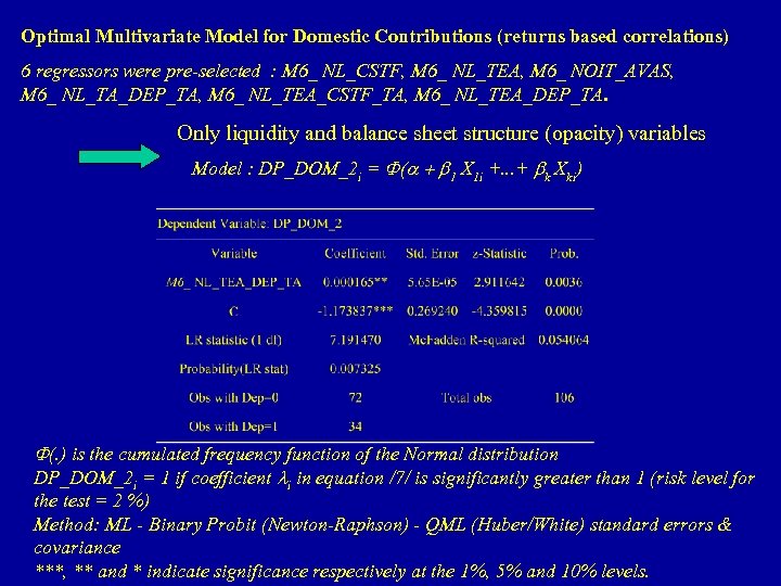
Optimal Multivariate Model for Domestic Contributions (returns based correlations) 6 regressors were pre-selected : M 6_ NL_CSTF, M 6_ NL_TEA, M 6_ NOIT_AVAS, M 6_ NL_TA_DEP_TA, M 6_ NL_TEA_CSTF_TA, M 6_ NL_TEA_DEP_TA. Only liquidity and balance sheet structure (opacity) variables Model : DP_DOM_2 i = F(a + b 1 X 1 i +. . . + bk Xki) F(. ) is the cumulated frequency function of the Normal distribution DP_DOM_2 i = 1 if coefficient li in equation /7/ is significantly greater than 1 (risk level for the test = 2 %) Method: ML - Binary Probit (Newton-Raphson) - QML (Huber/White) standard errors & covariance ***, ** and * indicate significance respectively at the 1%, 5% and 10% levels.
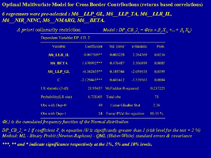
Optimal Multivariate Model for Cross Border Contributions (returns based correlations) 6 regressors were pre-selected : M 6__LLP_GL, M 6__LLP_TA, M 6__LLR_IL, M 6__NIR_NINC, M 6__NMARG, M 6__BETA. A priori colinearity restriction Model : DP_CB_2 i = F(a + b 1 X 1 i +. . . + bk Xki) F(. ) is the cumulated frequency function of the Normal distribution DP_CB_2 i = 1 if coefficient l'i in equation /8/ is significantly greater than 1 (risk level for the test = 2 %) Method: ML - Binary Probit (Newton-Raphson) - QML (Huber/White) standard errors & covariance ***, ** and * indicate significance respectively at the 1%, 5% and 10% levels.

ROBUSTNESS CHECKS • Pre-selecting variables (simple probit estimations) : to avoid the consequences of outliers, standard deviations of coefficients were bootstraped (1000 times). • Optimal multivariate probit model selected by stepwise ascending method : we checked for other methods (backward, forward) • We check for the consequences of multicolinearity on the optimal model specification by producing a Farar – Glauber test for the null of no colinearity. If it comes that the P-Value for the test does not exceed 50 % (colinearity presumption), we introduce a restriction in the stepwise process that renders such a result impossible

ROBUSTNESS CHECKS (continued) • We check for the optimal model DP_DOM_2 i = F(a + b 1 X 1 i +. . . + bk Xki) stability by testing the null a' = b 1' =. . . = bk' = 0 in the augmented model : DP_CB_2 i = F(a + b 1 X 1 i +. . . + bk Xki + a' Di + b 1' X 1 i Di +. . . + bk' Xki Di) where Di is a dummy for Bank type, Bank Nationality, bank country rank, bank world rank • Estimation of multivariate panel data fixed effect model considering a continuous dependent variable instead of the binary variable. In such a case, the values of the dependant variable are the annual means of country P domestic correlations ; the regressors values are, alternatively, the value of the accounting ratio j of the bank i at the end of the year t or the mean value of the market indicator j of bank i evaluated on the whole year t.
CONCLUSION • Average pair-wise correlations significantly differ among countries and the probability that a specific shock spreads to other banks has different determinants • Cross country bank contagion risk is better predicted by asset risk indicators whereas domestic contagion risk is better predicted by illiquidity and the extent of traditional intermediation activities (non tradable loans) which are opaque. • Our findings suggest that whereas illiquidity, but not insolvency, is a major concern at the domestic level the opposite is true for cross-country contagion. • Illiquidity could be a concern for cross border spillovers but only to a limited extent for large banks.
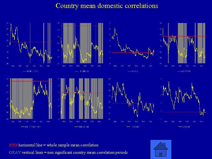
Country mean domestic correlations RED horizontal line = whole sample mean correlation GRAY vertical lines = non significant country mean correlation periods
9e452fa124f7590fe108edeac81303be.ppt