Housing Demand Supply Today Return Exam

Housing Demand Supply

Today • Return Exam • Second Paper – Discussion • Housing Services and Supply

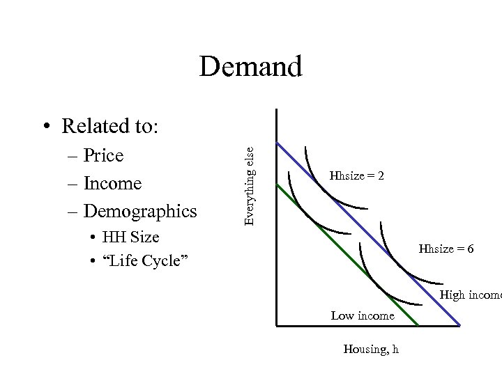Demand – Price – Income – Demographics Everything else • Related to: Hhsize = 2 • HH Size • “Life Cycle” Hhsize = 6 High income Low income Housing, h

Income Elasticities • If our income increases by $500, do we move? Why? • Economists feel that the appropriate measure to use is “permanent income, ” related to wealth. • Permanent income elasticities are probably somewhere between 0. 5 and 1. 0. Best guess may be 0. 5 to 0. 7. Discuss.

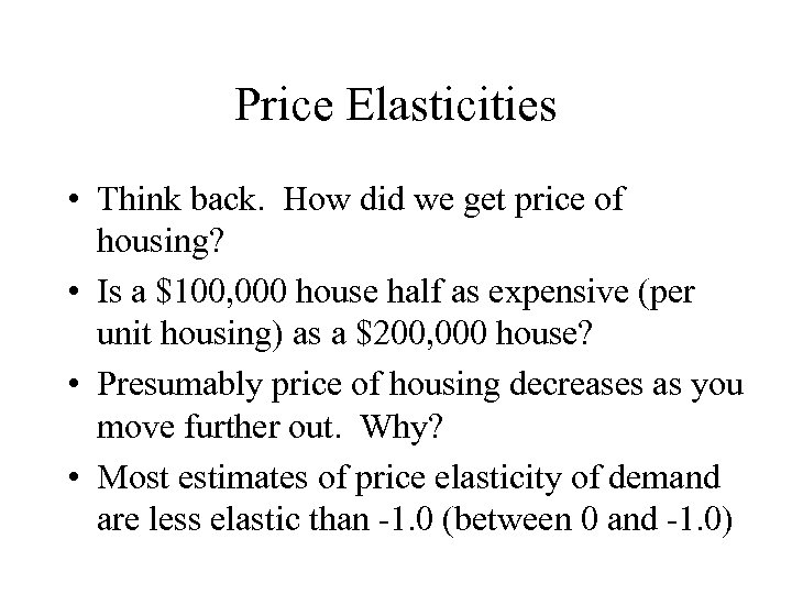Price Elasticities • Think back. How did we get price of housing? • Is a $100, 000 house half as expensive (per unit housing) as a $200, 000 house? • Presumably price of housing decreases as you move further out. Why? • Most estimates of price elasticity of demand are less elastic than -1. 0 (between 0 and -1. 0)

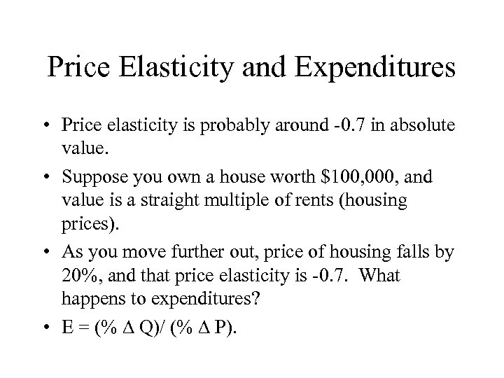Price Elasticity and Expenditures • Price elasticity is probably around -0. 7 in absolute value. • Suppose you own a house worth $100, 000, and value is a straight multiple of rents (housing prices). • As you move further out, price of housing falls by 20%, and that price elasticity is -0. 7. What happens to expenditures? • E = (% D Q)/ (% D P).

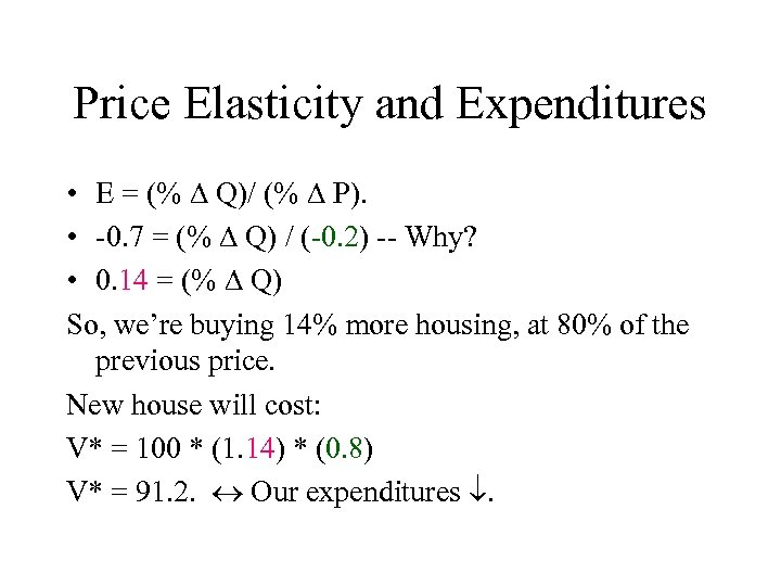Price Elasticity and Expenditures • E = (% D Q)/ (% D P). • -0. 7 = (% D Q) / (-0. 2) -- Why? • 0. 14 = (% D Q) So, we’re buying 14% more housing, at 80% of the previous price. New house will cost: V* = 100 * (1. 14) * (0. 8) V* = 91. 2. Our expenditures .

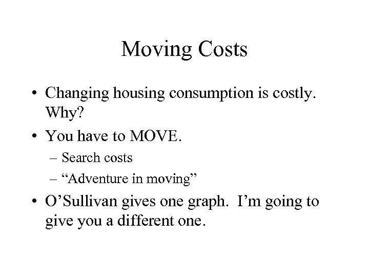Moving Costs • Changing housing consumption is costly. Why? • You have to MOVE. – Search costs – “Adventure in moving” • O’Sullivan gives one graph. I’m going to give you a different one.

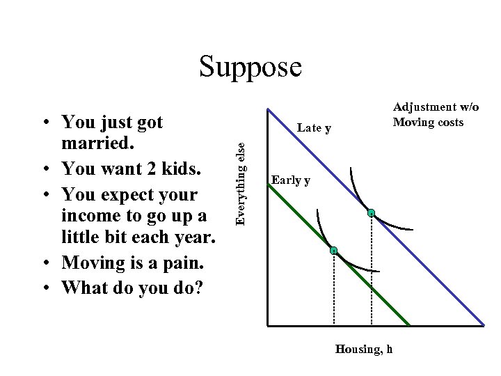Suppose Late y Everything else • You just got married. • You want 2 kids. • You expect your income to go up a little bit each year. • Moving is a pain. • What do you do? Adjustment w/o Moving costs Early y Housing, h

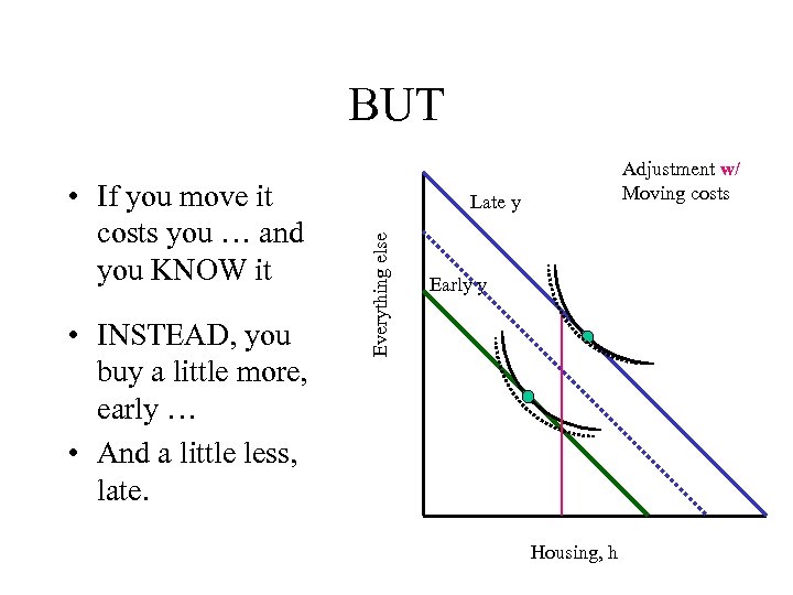BUT • INSTEAD, you buy a little more, early … • And a little less, late. Late y Everything else • If you move it costs you … and you KNOW it Adjustment w/ Moving costs Early y Housing, h

What happens? • You avoid the moving costs. • Point here, is that households don’t move every time their incomes change … • Or every time the housing price changes. • We want a story that is realistic.

Supply • Think, for now, of housing as entirely rental stock. • What do we know? – It is durable. Dwellings can last for 100 years or more. – Most of our housing supply comes from “used” stock, rather than new stock. – Supply of services is pretty inelastic. Only 2 to 3% of the housing on the market in any year is new.

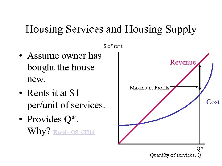Housing Services and Housing Supply $ of rent • Assume owner has bought the house new. • Rents it at $1 per/unit of services. • Provides Q*. Why? Excel - OS_CH 14 Revenue Maximum Profits Cost Q* Quantity of services, Q

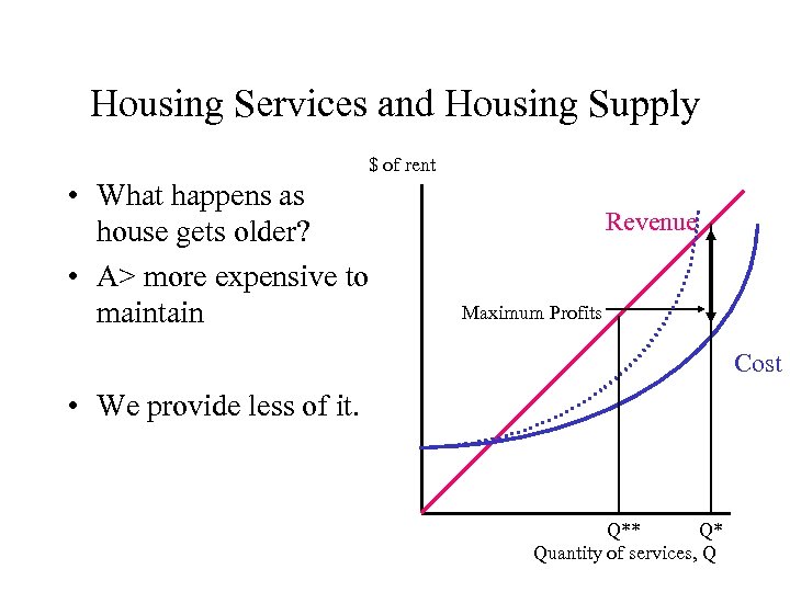Housing Services and Housing Supply $ of rent • What happens as house gets older? • A> more expensive to maintain Revenue Maximum Profits Cost • We provide less of it. Q** Q* Quantity of services, Q

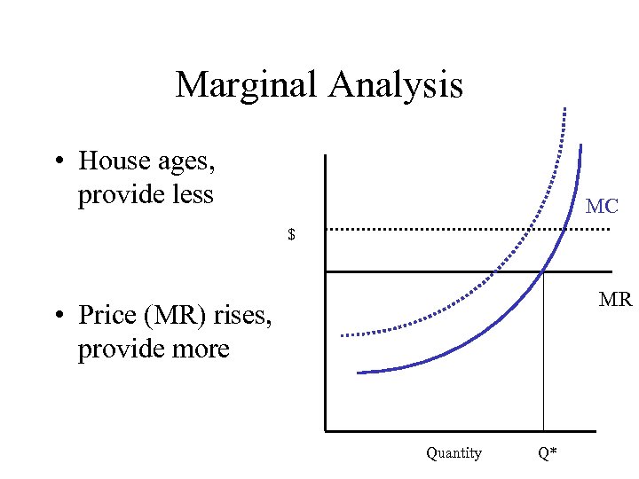Marginal Analysis • House ages, provide less MC $ MR • Price (MR) rises, provide more Quantity Q*

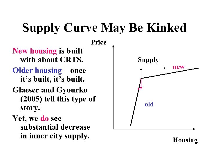Supply Curve May Be Kinked Price New housing is built with about CRTS. Older housing – once it’s built, it’s built. Glaeser and Gyourko (2005) tell this type of story. Yet, we do see substantial decrease in inner city supply. Supply new old Housing

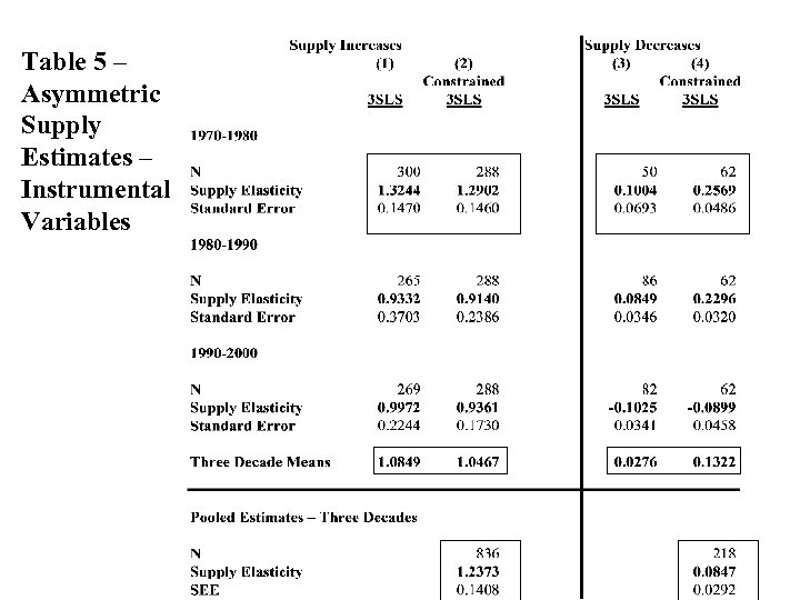Table 5 – Asymmetric Supply Estimates – Instrumental Variables

Sources Goodman, Allen C. , “The Other Side of Eight Mile, ” Real Estate Economics 33 (2005): 539569 Goodman, Allen C. , “Central Cities and Housing Supply: Growth and Decline in U. S. Cities, ” Journal of Housing Economics 14 (December 2005): 315 -335