a4dfca61c2048105a0580be4932a0cbc.ppt
- Количество слайдов: 59
HL Distributed Hydrologic Modeling Mike Smith Victor Koren, Seann Reed, Ziya Zhang, Fekadu Moreda, Fan Lei, Zhengtao Cui, Dongjun Seo, Shuzheng Cong, John Schaake DSST Feb 24, 2006 1
Overview • Today: – Goals, expectations, applicability – R&D • Next Call – Development Strategy – Implementation – RFC experiences 2
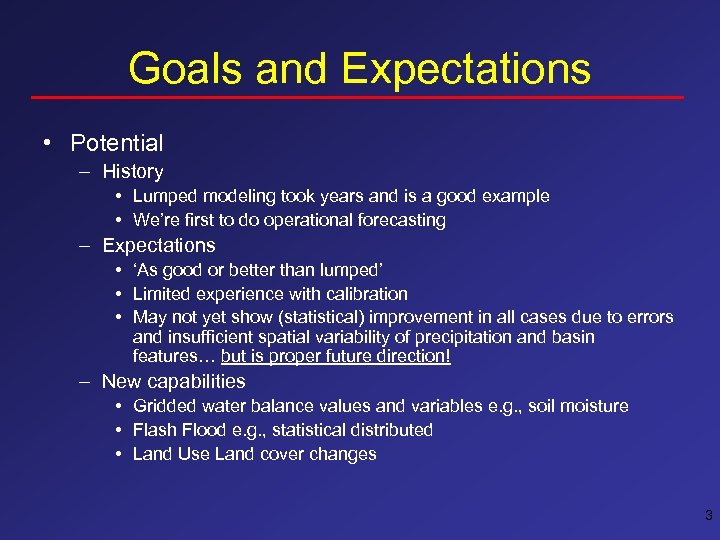
Goals and Expectations • Potential – History • Lumped modeling took years and is a good example • We’re first to do operational forecasting – Expectations • ‘As good or better than lumped’ • Limited experience with calibration • May not yet show (statistical) improvement in all cases due to errors and insufficient spatial variability of precipitation and basin features… but is proper future direction! – New capabilities • Gridded water balance values and variables e. g. , soil moisture • Flash Flood e. g. , statistical distributed • Land Use Land cover changes 3
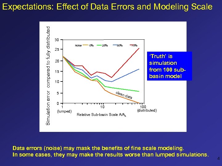
Simulation error compared to fully distributed Relative error, Ek, % Expectations: Effect of Data Errors and Modeling Scale 30 Noise 0% 25% 50% 75% 25 ‘Truth’ is simulation from 100 subbasin model 20 15 10 clea 5 0 1 (lumped) n da 10 ta 100 (distributed) Relative Sub-basin Scale A/Ak Data errors (noise) may mask the benefits of fine scale modeling. In some cases, they make the results worse than lumped simulations. 4
Goals and Expectations Rationale • Scientific motivation – Finer scales > better results – Data availability • Field requests • NOAA Water Resources Program • NIDIS 5
Goals and Expectations Applicability • Distributed models applicable everywhere • Issues – Data availability and quality needed to realize benefits – Parameterization – Calibration 6
Goals and Expectations Measures of Improvement • Hydrographs at points (DMIP 1) – Guidance from RFC • Spatial – Runoff – Soil moisture – Point to grid 7
HL R&D Strategy Goal: produce models, tools, guidelines to improve field office operations • Conduct in-house work • Collaborate with partners – U. Arizona, Penn St. University – DMIP 1, 2 – ETL • Work closely with RFC prototypes – ABRFC, WGRFC: DMS 1. 0 – MARFC, CBRFC: in-house • Publish results • NAS Review of AHPS Science 8
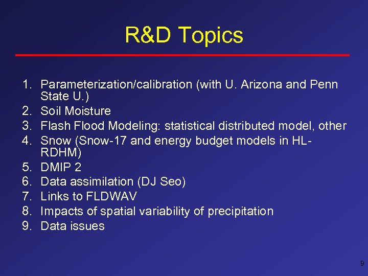
R&D Topics 1. Parameterization/calibration (with U. Arizona and Penn State U. ) 2. Soil Moisture 3. Flash Flood Modeling: statistical distributed model, other 4. Snow (Snow-17 and energy budget models in HLRDHM) 5. DMIP 2 6. Data assimilation (DJ Seo) 7. Links to FLDWAV 8. Impacts of spatial variability of precipitation 9. Data issues 9
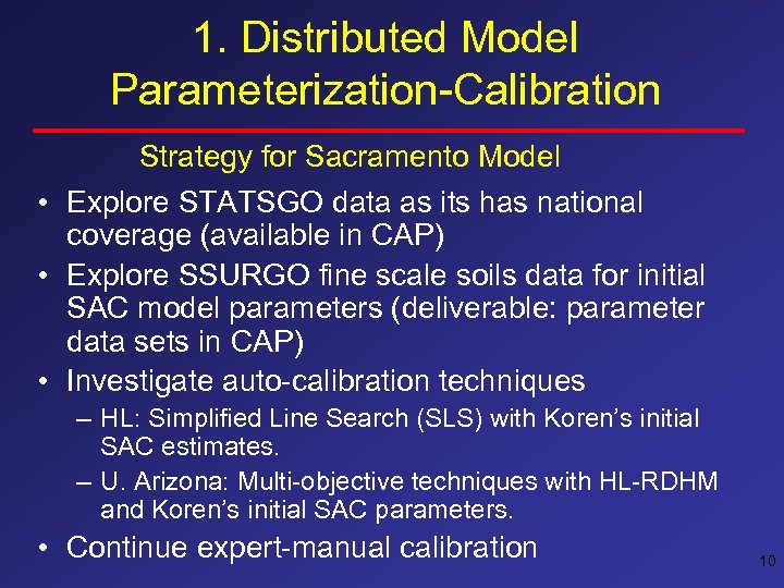
1. Distributed Model Parameterization-Calibration Strategy for Sacramento Model • Explore STATSGO data as its has national coverage (available in CAP) • Explore SSURGO fine scale soils data for initial SAC model parameters (deliverable: parameter data sets in CAP) • Investigate auto-calibration techniques – HL: Simplified Line Search (SLS) with Koren’s initial SAC estimates. – U. Arizona: Multi-objective techniques with HL-RDHM and Koren’s initial SAC parameters. • Continue expert-manual calibration 10
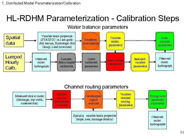
1. Distributed Model Parameterization/Calibration HL-RDHM Parameterization - Calibration Steps Water balance parameters Spatial data Lumped Hourly Calb. Variable basin properties (STATSGO 1 x 1 km grids: Soil texture, Hydrologic Soil Group, Land cover/use) Observed outlet hydrograph Lumped, Semi-lumped calibration Transform. relationships Variable model parameters Outlet calibrated parameters Area average parameters Scale adjusted parameters Rescaled variable parameters Observed outlet hydrograph Channel routing parameters Measured data at outlet (discharge, top width, cross-section) Channel routing parameters at outlets Geomorphological relations Spatially variable basin properties (slope, area, drainage density) Variable channel routing parameters Fitting curve parameter adjustment Observed outlet hydrographs 11
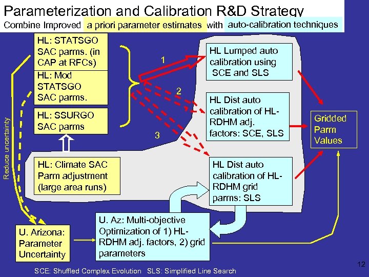
Parameterization and Calibration R&D Strategy auto-calibration techniques a priori parameter estimates Combine Improved a priori parameter estimates with Auto-calibration techniques Reduce uncertainty HL: STATSGO SAC parms. (in CAP at RFCs) HL: Mod STATSGO SAC parms. HL: SSURGO SAC parms HL Lumped auto calibration using SCE and SLS 1 2 3 HL: Climate SAC Parm adjustment (large area runs) U. Arizona: Parameter Uncertainty HL Dist auto calibration of HLRDHM adj. factors: SCE, SLS Gridded Parm Values HL Dist auto calibration of HLRDHM grid parms: SLS U. Az: Multi-objective Optimization of 1) HLRDHM adj. factors, 2) grid parameters SCE: Shuffled Complex Evolution SLS: Simplified Line Search 12
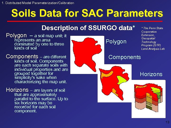
1. Distributed Model Parameterization/Calibration Soils Data for SAC Parameters Description of SSURGO data* Polygon – a soil map unit; it represents an area dominated by one to three kinds of soil Components – are different kinds of soil. Components are each separate soils with individual properties and are grouped together for simplicity's sake when characterizing the map unit. * The Penn State Cooperative Extension, Geospatial Technology Program (GTP) Land Analysis Lab Polygon Components Horizons – are layers of soil that are approximately parallel to the surface. Up to six horizons may be recorded for each soil component. 13
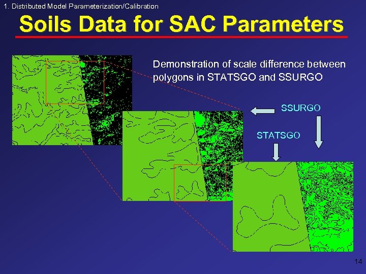
1. Distributed Model Parameterization/Calibration Soils Data for SAC Parameters Demonstration of scale difference between polygons in STATSGO and SSURGO STATSGO 14
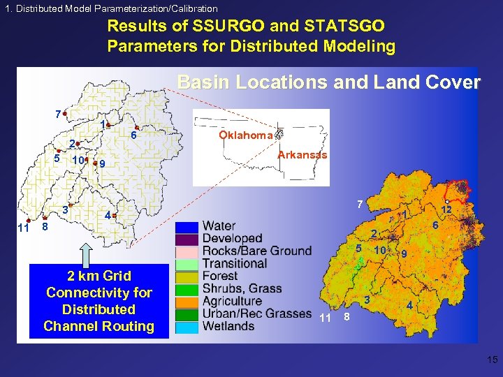
1. Distributed Model Parameterization/Calibration Results of SSURGO and STATSGO Parameters for Distributed Modeling Basin Locations and Land Cover 7 1 2 5 10 3 11 8 6 9 Oklahoma Arkansas 7 4 2 km Grid Connectivity for Distributed Channel Routing 1 2 5 10 3 11 8 12 6 9 4 15
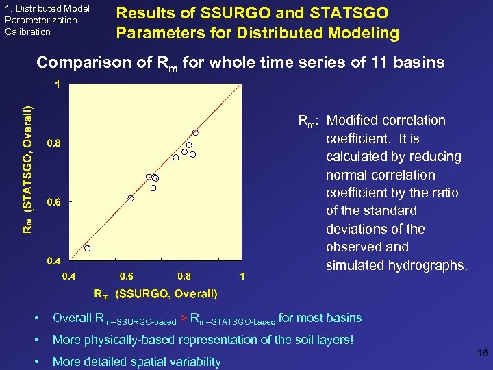
1. Distributed Model Parameterization Calibration Results of SSURGO and STATSGO Parameters for Distributed Modeling Comparison of Rm for whole time series of 11 basins Rm: Modified correlation coefficient. It is calculated by reducing normal correlation coefficient by the ratio of the standard deviations of the observed and simulated hydrographs. • Overall Rm--SSURGO-based > Rm--STATSGO-based for most basins • More physically-based representation of the soil layers! • More detailed spatial variability 16
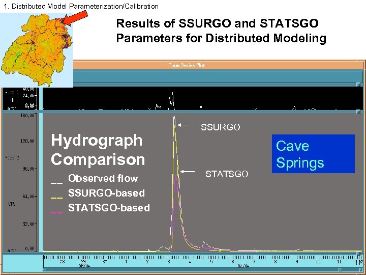
1. Distributed Model Parameterization/Calibration Results of SSURGO and STATSGO Parameters for Distributed Modeling Hydrograph Comparison __ Observed flow __ SSURGO-based __ STATSGO-based SSURGO STATSGO Cave Springs 17
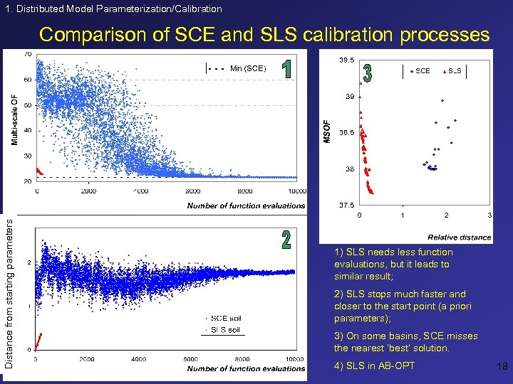
1. Distributed Model Parameterization/Calibration Distance from starting parameters Comparison of SCE and SLS calibration processes 1) SLS needs less function evaluations, but it leads to similar result; 2) SLS stops much faster and closer to the start point (a priori parameters); 3) On some basins, SCE misses the nearest ‘best’ solution. 4) SLS in AB-OPT 18
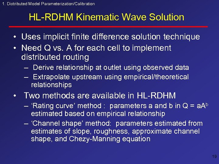
1. Distributed Model Parameterization/Calibration HL-RDHM Kinematic Wave Solution • Uses implicit finite difference solution technique • Need Q vs. A for each cell to implement distributed routing – Derive relationship at outlet using observed data – Extrapolate upstream using empirical/theoretical relationships • Two methods are available in HL-RDHM – ‘Rating curve’ method : parameters a and b in Q = a. Ab estimated based on empirical relationship – ‘Channel shape’ method: parameters estimated from estimates of slope, roughness, approximate channel shape, and Chezy-Manning equation 19
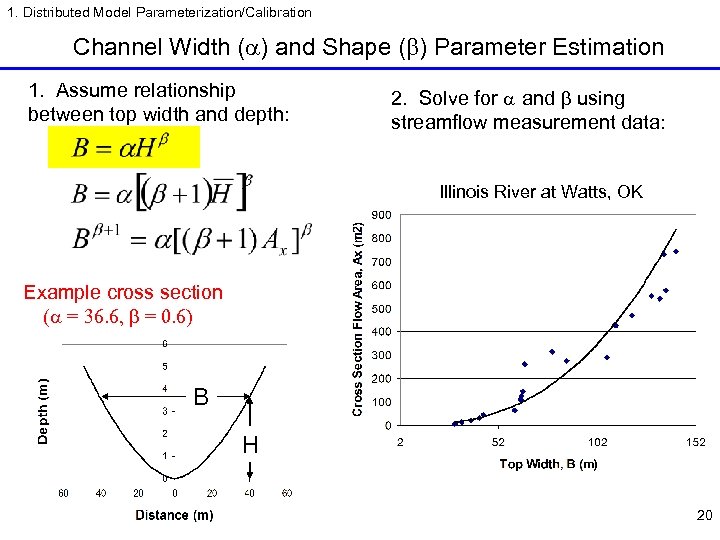
1. Distributed Model Parameterization/Calibration Channel Width (a) and Shape (b) Parameter Estimation 1. Assume relationship between top width and depth: 2. Solve for a and b using streamflow measurement data: Illinois River at Watts, OK Example cross section (a = 36. 6, b = 0. 6) B H 20
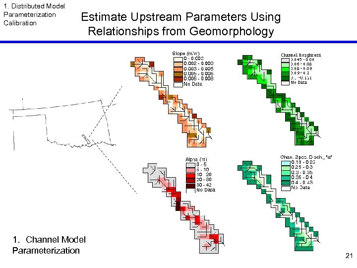
1. Distributed Model Parameterization Calibration Estimate Upstream Parameters Using Relationships from Geomorphology 1. Channel Model Parameterization 21
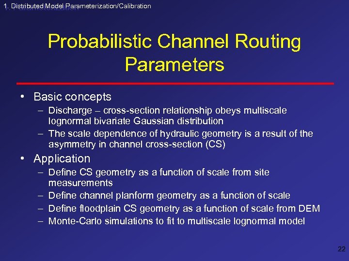
1. Distributed Model Parameterization/Calibration 1. Parameterization Probabilistic Channel Routing Parameters • Basic concepts – Discharge – cross-section relationship obeys multiscale lognormal bivariate Gaussian distribution – The scale dependence of hydraulic geometry is a result of the asymmetry in channel cross-section (CS) • Application – Define CS geometry as a function of scale from site measurements – Define channel planform geometry as a function of scale – Define floodplain CS geometry as a function of scale from DEM – Monte-Carlo simulations to fit to multiscale lognormal model 22
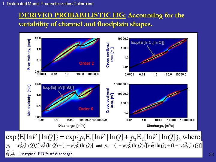
1. Distributed Model Parameterization/Calibration DERIVED PROBABILISTIC HG: Accounting for the variability of channel and floodplain shapes. Exp{E[ln. CA|ln. Q]} Exp{E[ln. V|ln. Q]} marginal PDFs of discharge 23
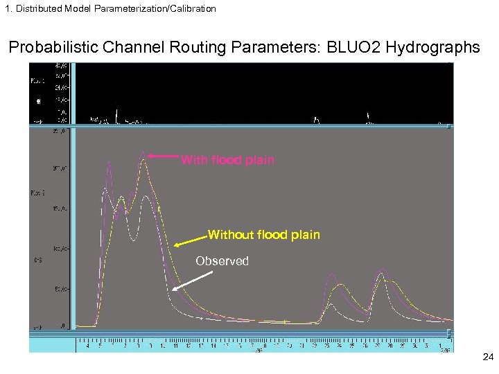
1. Distributed Model Parameterization/Calibration Probabilistic Channel Routing Parameters: BLUO 2 Hydrographs With flood plain Without flood plain Observed 24
2. Soil Moisture 2. Distributed Modeling and Soil Moisture • Use for calibration, verification of models • New products and services – NCRFC: WFO request – OHRFC: initialize MM 5 – NIDIS – NOAA Water Resources 25
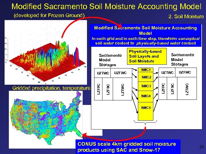
Modified Sacramento Soil Moisture Accounting Model (developed for Frozen Ground) 2. Soil Moisture Modified Sacramento Soil Moisture Accounting Model In each grid and in each time step, transform conceptual soil water content to physically-based water content Sacramento Model Storages UZTWC UZFWC Physically-based Soil Layers and Soil Moisture SMC 1 Sacramento Model Storages UZTWC UZFWC LZTWC SMC 4 LZFSC SMC 3 LZFPC LZTWC LZFSC Gridded precipitation, temperature LZFPC SMC 2 SMC 5 CONUS scale 4 km gridded soil moisture products using SAC and Snow-17 26
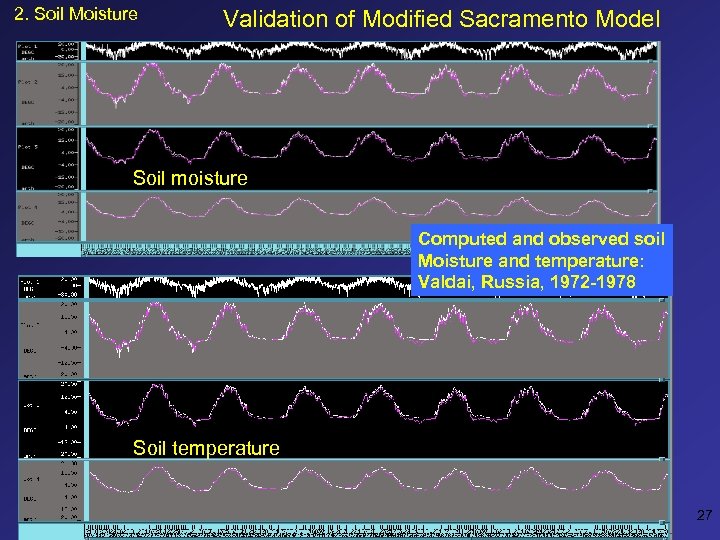
2. Soil Moisture Validation of Modified Sacramento Model Soil moisture Computed and observed soil Moisture and temperature: Valdai, Russia, 1972 -1978 Soil temperature 27
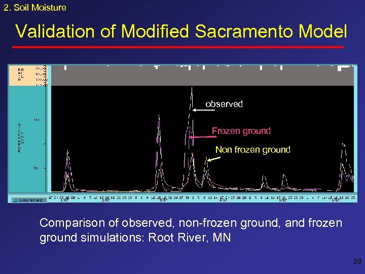
2. Soil Moisture Validation of Modified Sacramento Model observed Frozen ground Non frozen ground Comparison of observed, non-frozen ground, and frozen ground simulations: Root River, MN 28
2. Soil Moisture Modified SAC • Publications – Koren, 2005. “Physically-Based Parameterization of Frozen Ground Effects: Sensitivity to Soil Properties” VIIth IAHS Scientific Assembly, Session 7. 2, Brazil, April. – Koren, 2003. Parameterization of Soil Moisture-Heat Transfer Processes for Conceptual Hydrological Models”, paper EAE 03 -A-06486 HS 18 -1 TU 1 P 0390, AGU-EGU, Nice, France, April. – Mitchell, K. , Koren, others, 2002. “Reducing near-surface cool/moist biases over snowpack and early spring wet soils in NCEP ETA model forecasts via land surface model upgrades”, Paper J 1. 1, 16 th AMS Hydrology Conference, Orlando, Florida, January – Koren et al. , 1999. “A parameterization of snowpack and frozen ground intended for NCEP weather and climate models”, J. Geophysical Research, 104, D 16, 19, 569 -19, 585. – Koren, et al. , 1999. “Validation of a snow-frozen ground parameterization of the ETA model”, 14 th Conference on Hydrology, 10 -15 January 1999, Dallas, TX, by the AMS, Boston MA, pp. 410 -413. – http: //www. nws. noaa. gov/oh/hrl/frzgrd/index. html 29
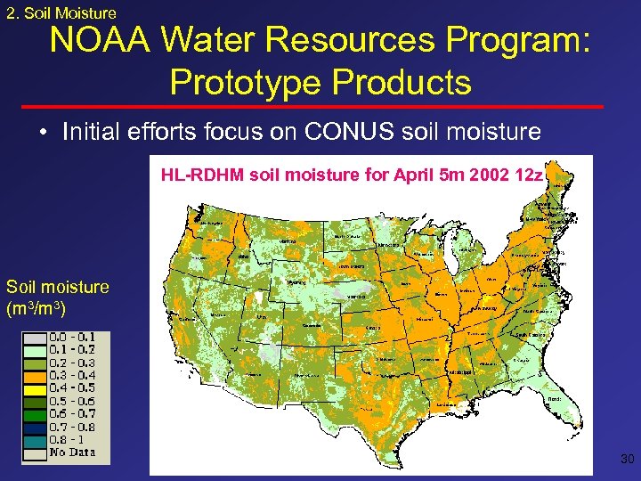
2. Soil Moisture NOAA Water Resources Program: Prototype Products • Initial efforts focus on CONUS soil moisture HL-RDHM soil moisture for April 5 m 2002 12 z Soil moisture (m 3/m 3) 30
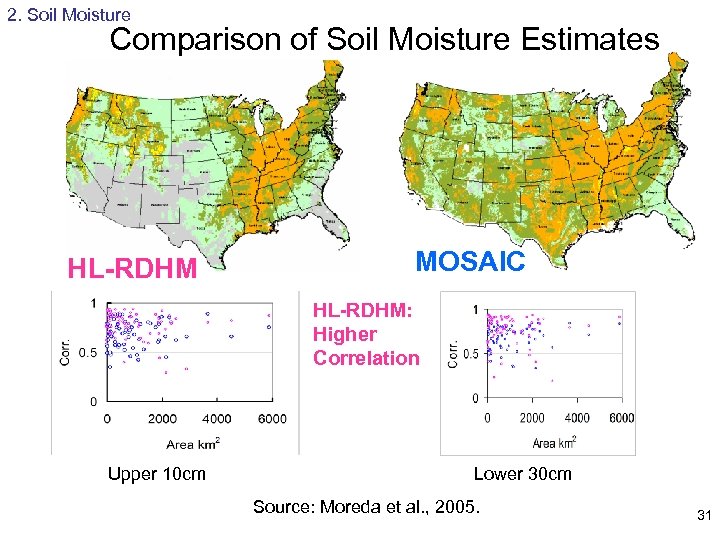
2. Soil Moisture Comparison of Soil Moisture Estimates HL-RDHM MOSAIC HL-RDHM: Higher Correlation Upper 10 cm Lower 30 cm Source: Moreda et al. , 2005. 31
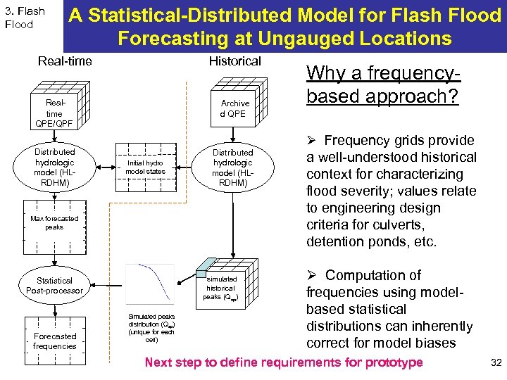
3. Flash Flood A Statistical-Distributed Model for Flash Flood Forecasting at Ungauged Locations Real-time Historical Realtime QPE/QPF Distributed hydrologic model (HLRDHM) Archive d QPE Ø Frequency grids provide Initial hydro model states Distributed hydrologic model (HLRDHM) Max forecasted peaks simulated historical peaks (Qsp) Statistical Post-processor Forecasted frequencies Why a frequencybased approach? Simulated peaks distribution (Qsp) (unique for each cell) a well-understood historical context for characterizing flood severity; values relate to engineering design criteria for culverts, detention ponds, etc. Ø Computation of frequencies using modelbased statistical distributions can inherently correct for model biases Next step to define requirements for prototype 32
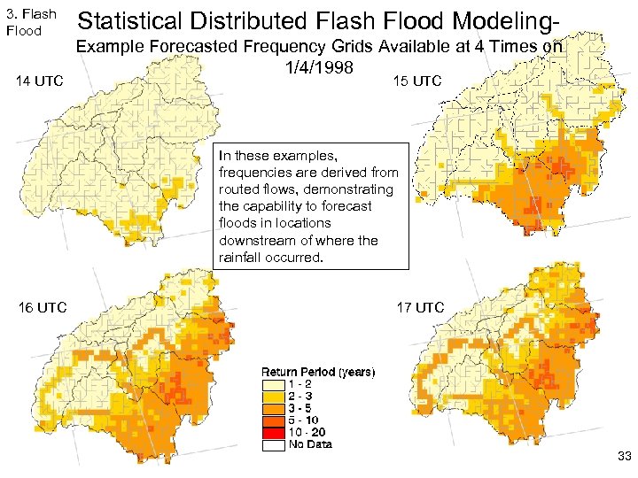
3. Flash Flood 14 UTC Statistical Distributed Flash Flood Modeling. Example Forecasted Frequency Grids Available at 4 Times on 1/4/1998 15 UTC In these examples, frequencies are derived from routed flows, demonstrating the capability to forecast floods in locations downstream of where the rainfall occurred. 16 UTC 17 UTC 33
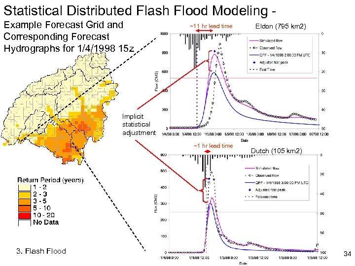
Statistical Distributed Flash Flood Modeling Example Forecast Grid and Corresponding Forecast Hydrographs for 1/4/1998 15 z ~11 hr lead time Eldon (795 km 2) Implicit statistical adjustment ~1 hr lead time 3. Flash Flood Dutch (105 km 2) 34
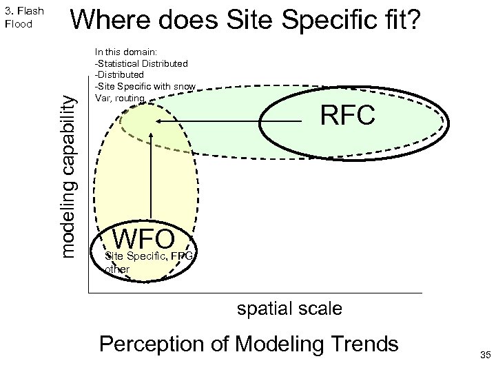
Where does Site Specific fit? modeling capability 3. Flash Flood In this domain: -Statistical Distributed -Site Specific with snow Var, routing RFC WFO Site Specific, FFG, other spatial scale Perception of Modeling Trends 35
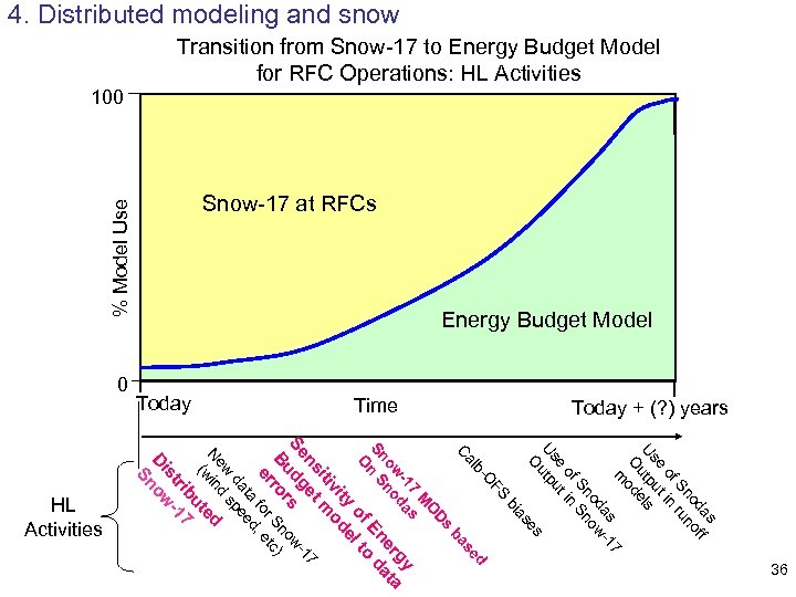
bi ed s ba as f od nof Sn ru of in e ut Us utp els O od m 7 as -1 od ow Sn Sn of in e ut Us p ut O es as FS O lb Ds O M 7 s -1 da gy ow no er ata Sn S En d n O of l to ty de o m Ca vi iti 36 ns et 17 Se dg s ow. Bu ror Sn c) er for , et ta ed da spe w d d Ne in (w ute rib 7 st -1 Di ow Sn HL Activities Today + (? ) years Time Today 0 Transition from Snow-17 to Energy Budget Model for RFC Operations: HL Activities 100 Snow-17 at RFCs Energy Budget Model % Model Use 4. Distributed modeling and snow
4. Distributed modeling and snow Distributed Snow-17 • Strategy: use distributed Snow-17 as a step in the migration to energy budget modeling: what can we learn? • Snow-17 now in HL-RDHM • Tested in MARFC area and over CONUS (delivered historical data) • Further testing in DMIP 2 • Gridded Snow-17 parameters for CONUS under review (could be delivered in CAP) • Related work: data needs for energy budget snow models 37
4. Distributed modeling and snow Current approach SNOW-17 model within HL-RDHM • SNOW-17 model is run at each pixel • Gridded precipitation from multi-sensor products are provided at each pixel • Gridded temperature inputs are provided by using DEM and regional temperature lapse rate • The area depletion curve is removed because of distributed approach • Other parameters are studied either to replace them with physical properties or relate them to these properties, e. g. , SCF. 38
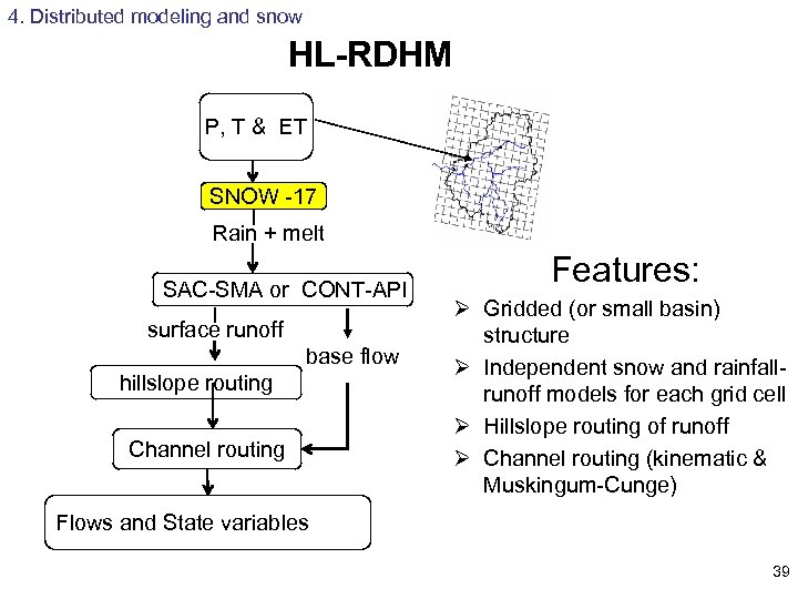
4. Distributed modeling and snow HL-RDHM P, T & ET SNOW -17 Rain + melt SAC-SMA or CONT-API surface runoff base flow hillslope routing Channel routing Features: Ø Gridded (or small basin) structure Ø Independent snow and rainfallrunoff models for each grid cell Ø Hillslope routing of runoff Ø Channel routing (kinematic & Muskingum-Cunge) Flows and State variables 39
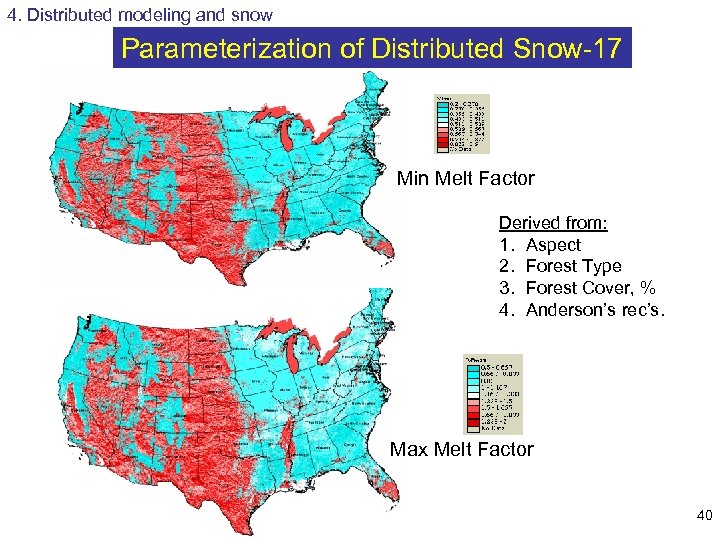
4. Distributed modeling and snow Parameterization of Distributed Snow-17 Min Melt Factor Derived from: 1. Aspect 2. Forest Type 3. Forest Cover, % 4. Anderson’s rec’s. Max Melt Factor 40
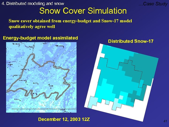
4. Distributed modeling and snow Snow Cover Simulation …Case Study Snow cover obtained from energy-budget and Snow-17 model qualitatively agree well Energy-budget model assimilated December 12, 2003 12 Z Distributed Snow-17 41
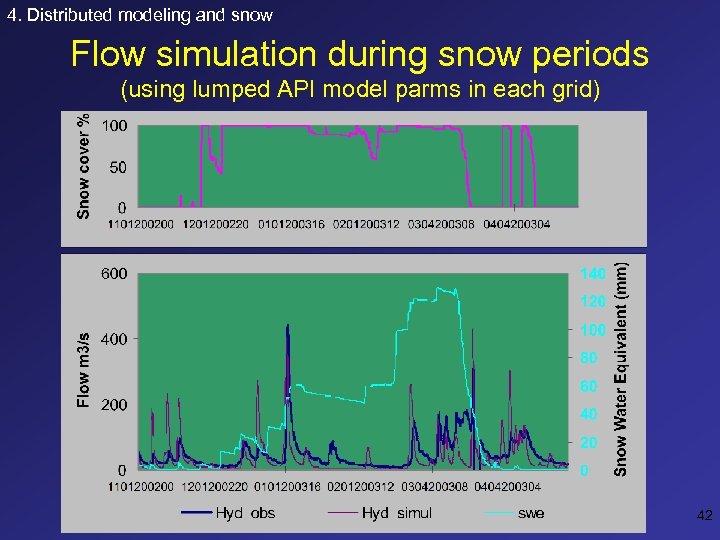
4. Distributed modeling and snow Flow simulation during snow periods (using lumped API model parms in each grid) 42
5. DMIP 2 – HL distributed model is worthy of implementation: we need to improve it for RFC use in all geographic regions – Partial funding from Water Resources – Much outside interest – HMT collaboration 43
5. DMIP 2 Science Questions • Confirm basic DMIP 1 conclusions with a longer validation period and more test basins • Improve our understanding of distributed model accuracy for small, interior point simulations: flash flood scenarios • Evaluate new forcing data sets (e. g. , HMT) • Evaluate the performance of distributed models in prediction mode • Use available soil moisture data to evaluate the physics of distributed models • Improve our understanding of the way routing schemes contribute to the success of distributed models • Continue to gain insights into the interplay among spatial variability in rainfall, physiographic features, and basin response, specifically in mountainous basins • Improve our understanding of scale/data issues in mountainous area hydrology • Improve our ability to characterize simulation and forecast uncertainty in different hydrologic regimes • Investigate data density/quality needs in mountainous areas (Georgakakos et al. , 1999; Tsintikidis, et al. , 2002) 44
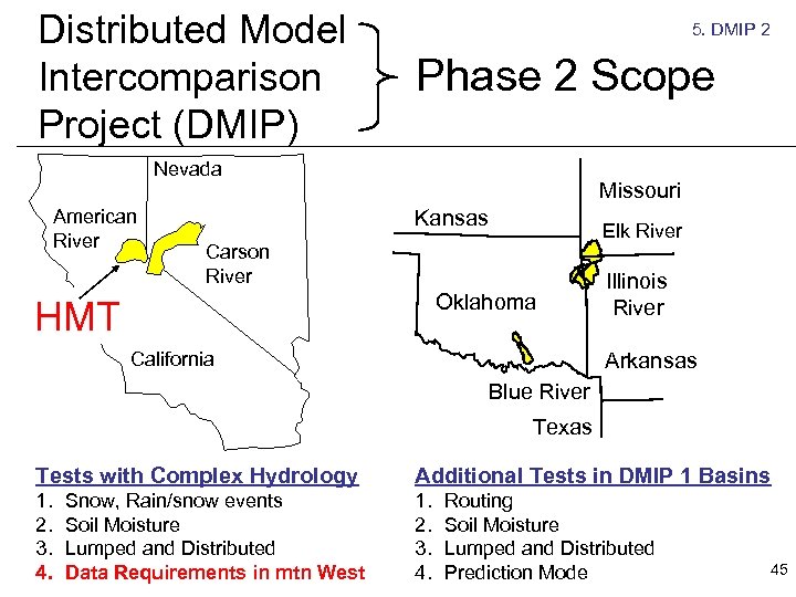
Distributed Model Intercomparison Project (DMIP) 5. DMIP 2 Phase 2 Scope Nevada American River Missouri Kansas Elk River Carson River Oklahoma HMT Illinois River Arkansas California Blue River Texas Tests with Complex Hydrology Additional Tests in DMIP 1 Basins 1. 2. 3. 4. Snow, Rain/snow events Soil Moisture Lumped and Distributed Data Requirements in mtn West Routing Soil Moisture Lumped and Distributed Prediction Mode 45
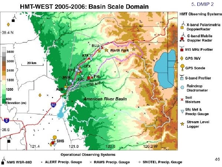
5. DMIP 2 46
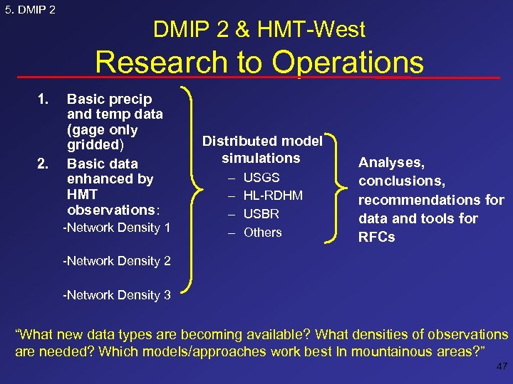
5. DMIP 2 & HMT-West Research to Operations 1. 2. Basic precip and temp data (gage only gridded) Basic data enhanced by HMT observations: -Network Density 1 Distributed model simulations – – USGS HL-RDHM USBR Others Analyses, conclusions, recommendations for data and tools for RFCs -Network Density 2 -Network Density 3 “What new data types are becoming available? What densities of observations are needed? Which models/approaches work best In mountainous areas? ” 47
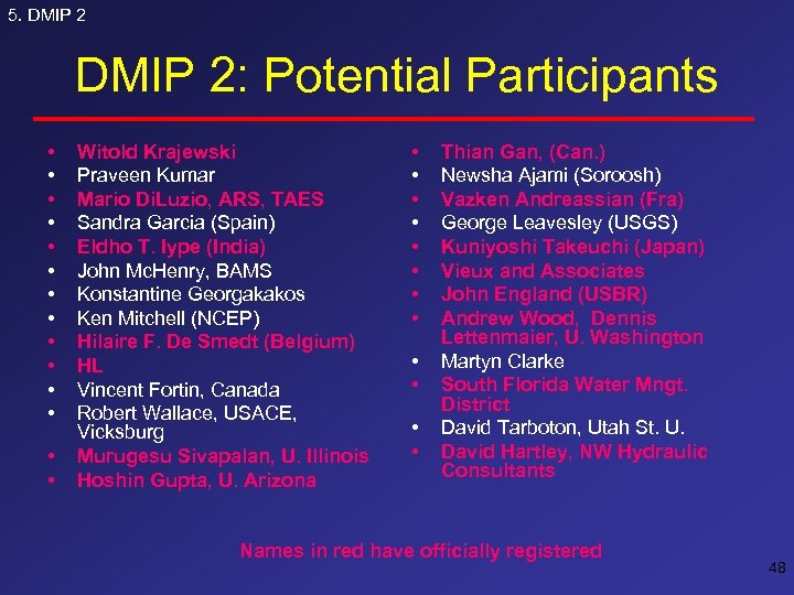
5. DMIP 2: Potential Participants • • • • Witold Krajewski Praveen Kumar Mario Di. Luzio, ARS, TAES Sandra Garcia (Spain) Eldho T. Iype (India) John Mc. Henry, BAMS Konstantine Georgakakos Ken Mitchell (NCEP) Hilaire F. De Smedt (Belgium) HL Vincent Fortin, Canada Robert Wallace, USACE, Vicksburg Murugesu Sivapalan, U. Illinois Hoshin Gupta, U. Arizona • • • Thian Gan, (Can. ) Newsha Ajami (Soroosh) Vazken Andreassian (Fra) George Leavesley (USGS) Kuniyoshi Takeuchi (Japan) Vieux and Associates John England (USBR) Andrew Wood, Dennis Lettenmaier, U. Washington Martyn Clarke South Florida Water Mngt. District David Tarboton, Utah St. U. David Hartley, NW Hydraulic Consultants Names in red have officially registered 48
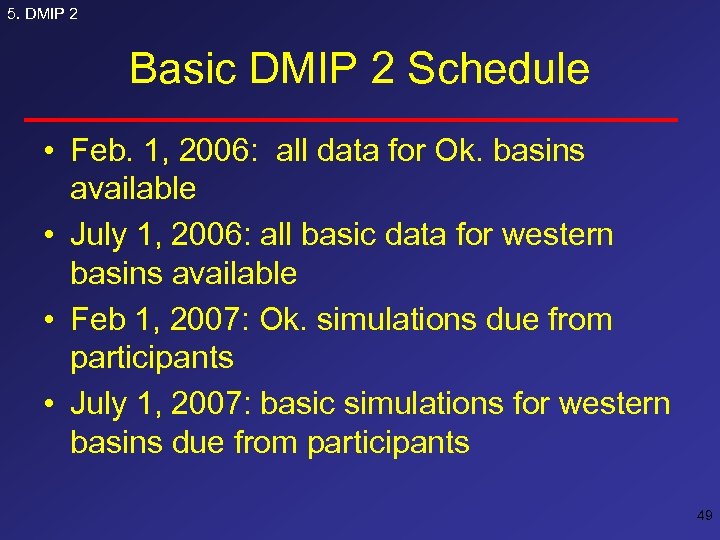
5. DMIP 2 Basic DMIP 2 Schedule • Feb. 1, 2006: all data for Ok. basins available • July 1, 2006: all basic data for western basins available • Feb 1, 2007: Ok. simulations due from participants • July 1, 2007: basic simulations for western basins due from participants 49
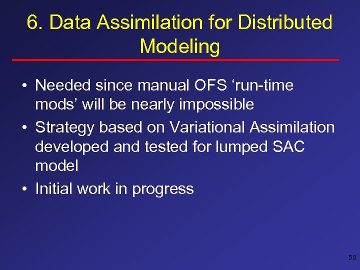
6. Data Assimilation for Distributed Modeling • Needed since manual OFS ‘run-time mods’ will be nearly impossible • Strategy based on Variational Assimilation developed and tested for lumped SAC model • Initial work in progress 50
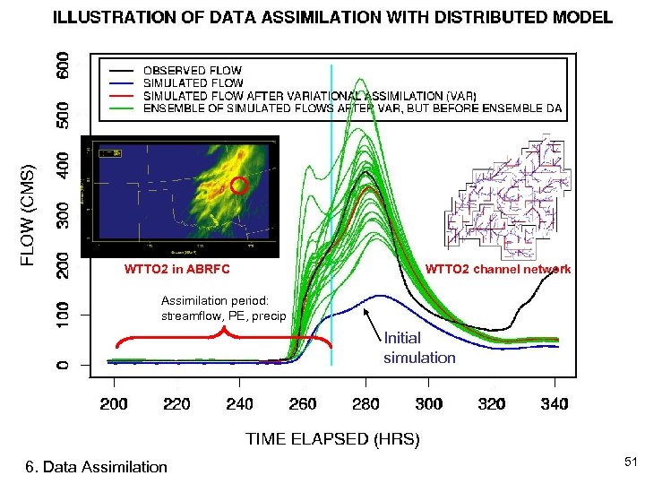
WTTO 2 in ABRFC WTTO 2 channel network Assimilation period: streamflow, PE, precip Initial simulation 6. Data Assimilation 51
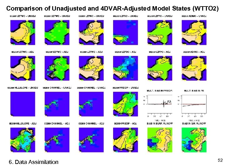
Comparison of Unadjusted and 4 DVAR-Adjusted Model States (WTTO 2) 6. Data Assimilation 52
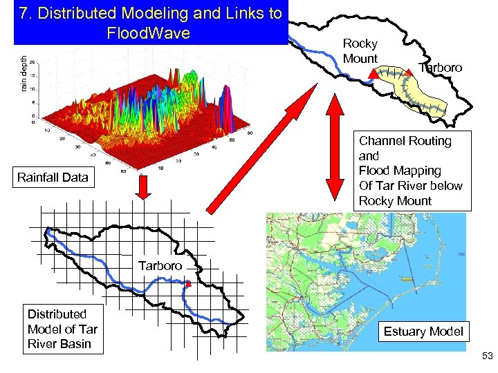
rain depth 7. Distributed Modeling and Links to Flood. Wave Rocky Mount Tarboro Channel Routing and Flood Mapping Of Tar River below Rocky Mount Rainfall Data Tarboro Distributed Model of Tar River Basin Estuary Model 53
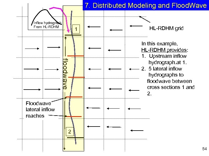
7. Distributed Modeling and Flood. Wave Inflow hydrograph From HL-RDHM 1 HL-RDHM grid floodwave In this example, HL-RDHM provides: 1. Upstream inflow hydrograph. at 1. 2. 5 lateral inflow hydrographs to floodwave between cross sections 1 and 2. Floodwave lateral inflow reaches 2 54
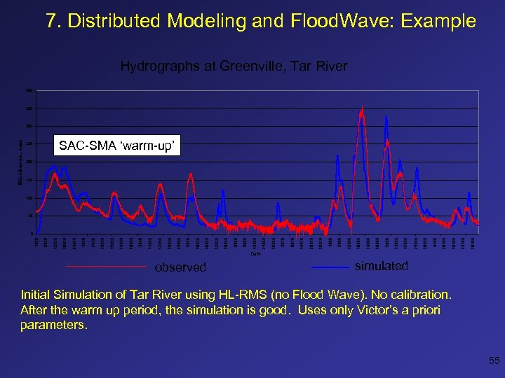
7. Distributed Modeling and Flood. Wave: Example Hydrographs at Greenville, Tar River 400 350 300 250 SAC-SMA ‘warm-up’ 200 150 100 50 0 Date observed simulated Initial Simulation of Tar River using HL-RMS (no Flood Wave). No calibration. After the warm up period, the simulation is good. Uses only Victor’s a priori parameters. 55
8. Impact of Spatial Variability • Question: how much spatial variability in precipitation and basin features is needed to warrant use of a distributed model? • Goal: provide guidance/tools to RFCs to help guide implementation of distributed models, i. e. , which basins will show most ‘bang for the buck’? • Initial tests completed after DMIP 1: trends seen but no clear ‘thresholds’ 56
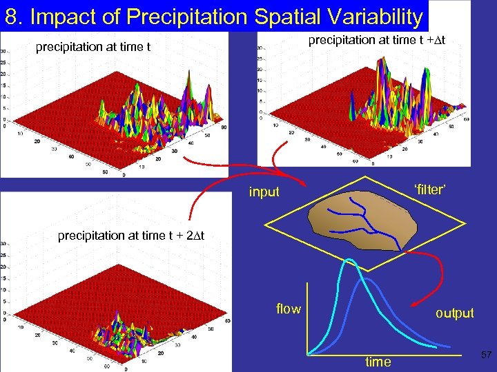
8. Impact of Precipitation Spatial Variability precipitation at time t +Dt precipitation at time t ‘filter’ input precipitation at time t + 2 Dt flow output time 57
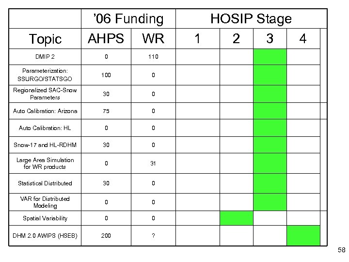
Topic ’ 06 Funding AHPS WR DMIP 2 0 110 Parameterization: SSURGO/STATSGO 100 0 Regionalized SAC-Snow Parameters 30 0 Auto Calibration: Arizona 75 0 Auto Calibration: HL 0 0 Snow-17 and HL-RDHM 30 0 Large Area Simulation for WR products 0 31 Statistical Distributed 30 0 VAR for Distributed Modeling 0 0 Spatial Variability 0 0 DHM 2. 0 AWIPS (HSEB) 200 HOSIP Stage 1 2 3 4 ? 58
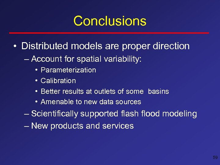
Conclusions • Distributed models are proper direction – Account for spatial variability: • • Parameterization Calibration Better results at outlets of some basins Amenable to new data sources – Scientifically supported flash flood modeling – New products and services 59
a4dfca61c2048105a0580be4932a0cbc.ppt