High School Mathematics at the Research Frontier Don

High School Mathematics at the Research Frontier Don Lincoln Fermilab http: //www-d 0. fnal. gov/~lucifer/Power. Point/HSMath. ppt

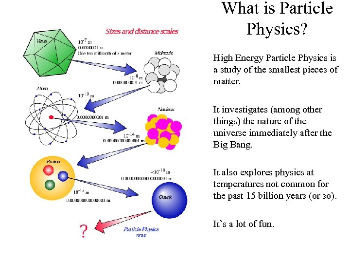What is Particle Physics? High Energy Particle Physics is a study of the smallest pieces of matter. It investigates (among other things) the nature of the universe immediately after the Big Bang. It also explores physics at temperatures not common for the past 15 billion years (or so). It’s a lot of fun.

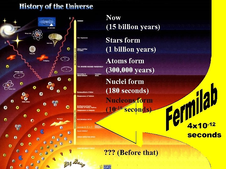Now (15 billion years) Stars form (1 billion years) Atoms form (300, 000 years) Nuclei form (180 seconds) Nucleons form (10 -10 seconds) 4 x 10 -12 seconds ? ? ? (Before that)

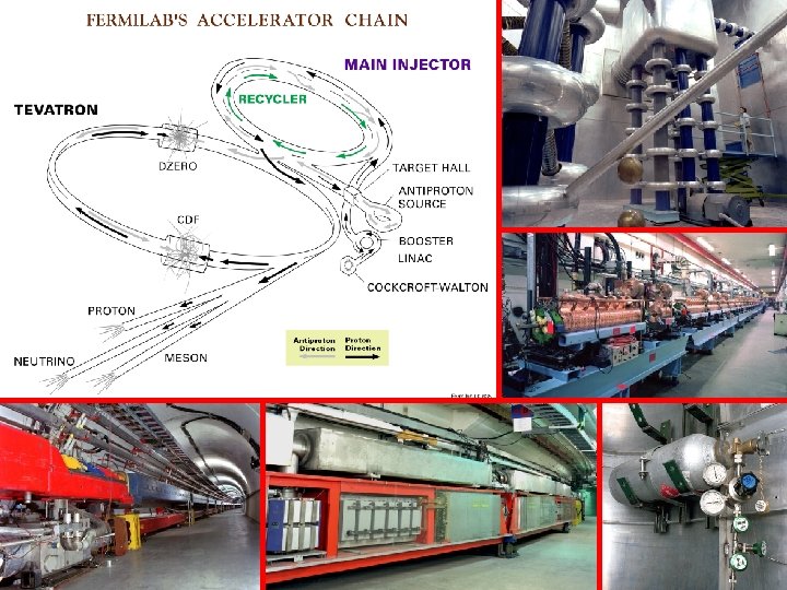
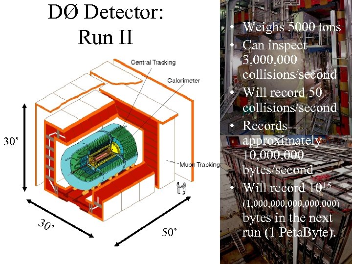DØ Detector: Run II 30’ • Weighs 5000 tons • Can inspect 3, 000 collisions/second • Will record 50 collisions/second • Records approximately 10, 000 bytes/second • Will record 1015 (1, 000, 000) 30 ’ 50’ bytes in the next run (1 Peta. Byte).

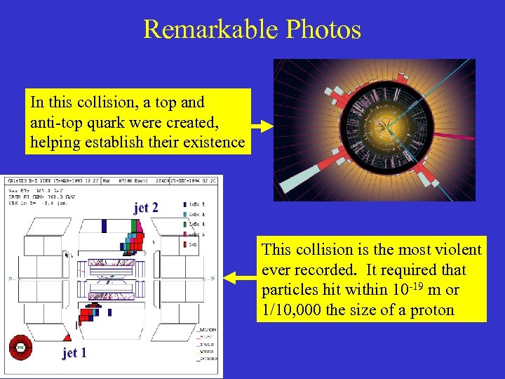Remarkable Photos In this collision, a top and anti-top quark were created, helping establish their existence This collision is the most violent ever recorded. It required that particles hit within 10 -19 m or 1/10, 000 the size of a proton

How Do You Measure Energy? • Go to Walmart and buy an energy detector? • Ask the guy sitting the next seat over and hope the teacher doesn’t notice? • Ignore the problem and spend the day on the beach? • Design and build your equipment and calibrate it yourself.

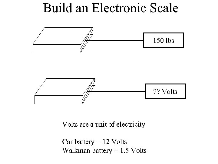Build an Electronic Scale 150 lbs ? ? Volts are a unit of electricity Car battery = 12 Volts Walkman battery = 1. 5 Volts

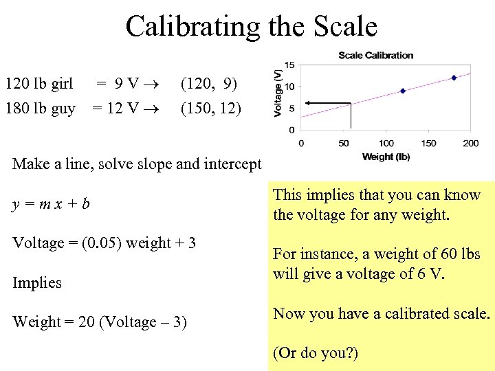Calibrating the Scale 120 lb girl 180 lb guy = 9 V = 12 V (120, 9) (150, 12) Make a line, solve slope and intercept y=mx+b Voltage = (0. 05) weight + 3 Implies Weight = 20 (Voltage – 3) This implies that you can know the voltage for any weight. For instance, a weight of 60 lbs will give a voltage of 6 V. Now you have a calibrated scale. (Or do you? )

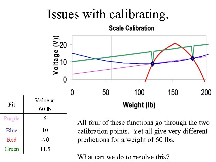Issues with calibrating. Fit Value at 60 lb Purple 6 Blue 10 Red -70 Green 11. 5 All four of these functions go through the two calibration points. Yet all give very different predictions for a weight of 60 lbs. What can we do to resolve this?

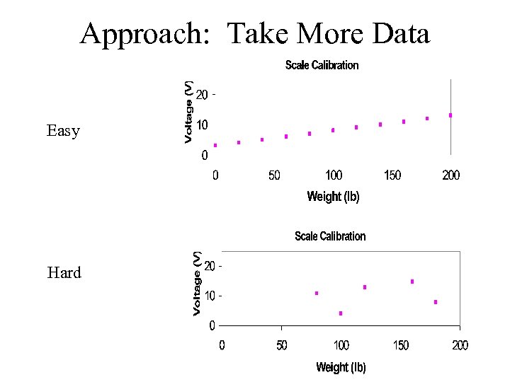Approach: Take More Data Easy Hard

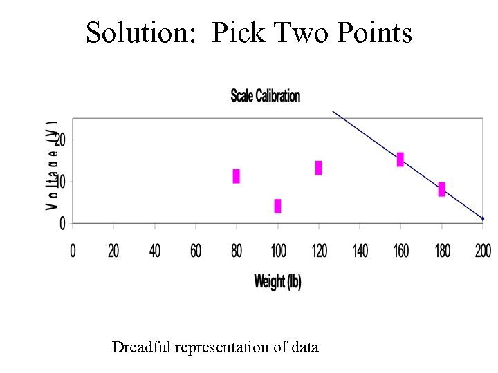Solution: Pick Two Points Dreadful representation of data

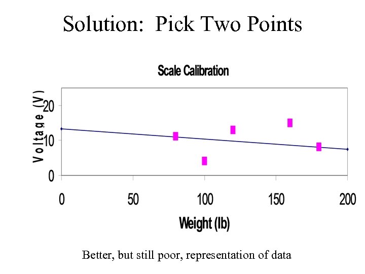Solution: Pick Two Points Better, but still poor, representation of data

Why don’t all the data lie on a line? • Error associated with each calibration point. • Must account for that in data analysis. • How do we determine errors? • What if some points have larger errors than others? How do we deal with this?

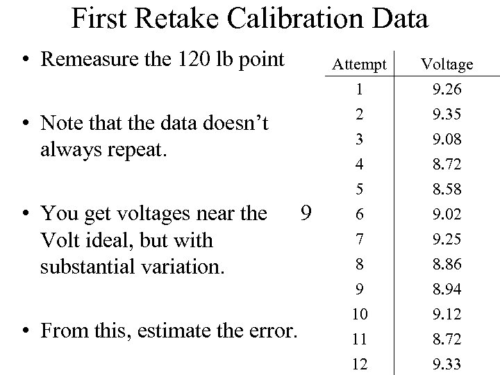First Retake Calibration Data • Remeasure the 120 lb point Attempt 1 2 3 • Note that the data doesn’t always repeat. • You get voltages near the Volt ideal, but with substantial variation. • From this, estimate the error. 9 Voltage 9. 26 9. 35 9. 08 4 5 6 7 8 9 10 11 8. 72 8. 58 9. 02 9. 25 8. 86 8. 94 9. 12 8. 72 12 9. 33

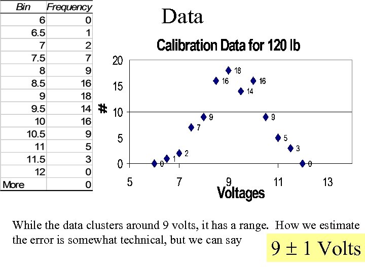Data While the data clusters around 9 volts, it has a range. How we estimate the error is somewhat technical, but we can say 9 1 Volts

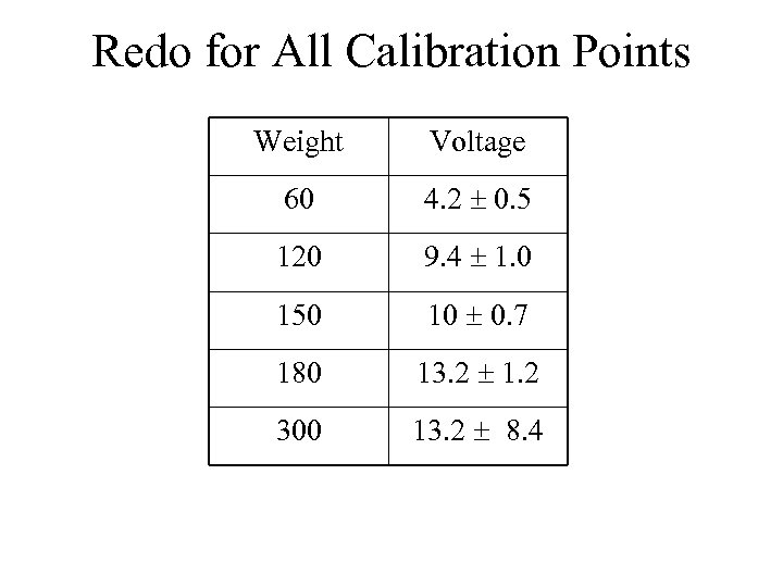Redo for All Calibration Points Weight Voltage 60 4. 2 0. 5 120 9. 4 1. 0 150 10 0. 7 180 13. 2 1. 2 300 13. 2 8. 4

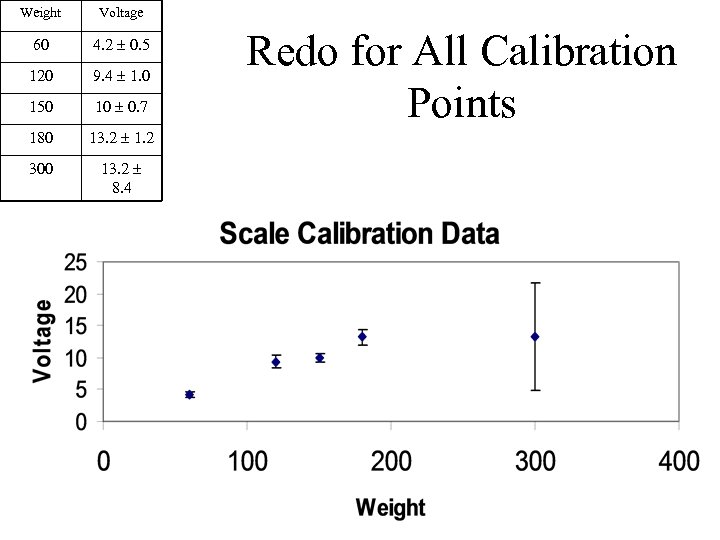Weight Voltage 60 4. 2 0. 5 120 9. 4 1. 0 150 10 0. 7 180 13. 2 1. 2 300 13. 2 8. 4 Redo for All Calibration Points

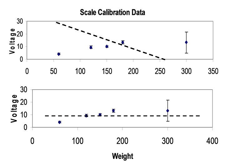
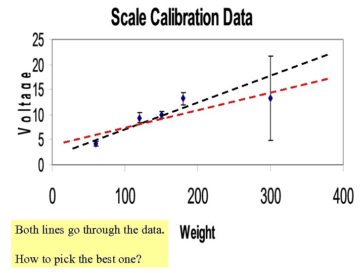Both lines go through the data. How to pick the best one?

State the Problem • How to use mathematical techniques to determine which line is best? • How to estimate the amount of variability allowed in the found slope and intercept that will also allow for a reasonable fit? • Answer will be m Dm and b Db

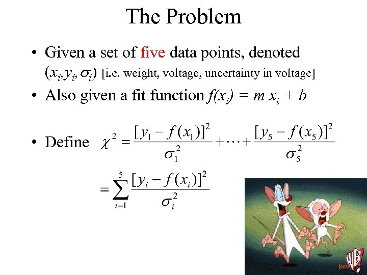The Problem • Given a set of five data points, denoted (xi, yi, si) [i. e. weight, voltage, uncertainty in voltage] • Also given a fit function f(xi) = m xi + b • Define Looks Intimidating!

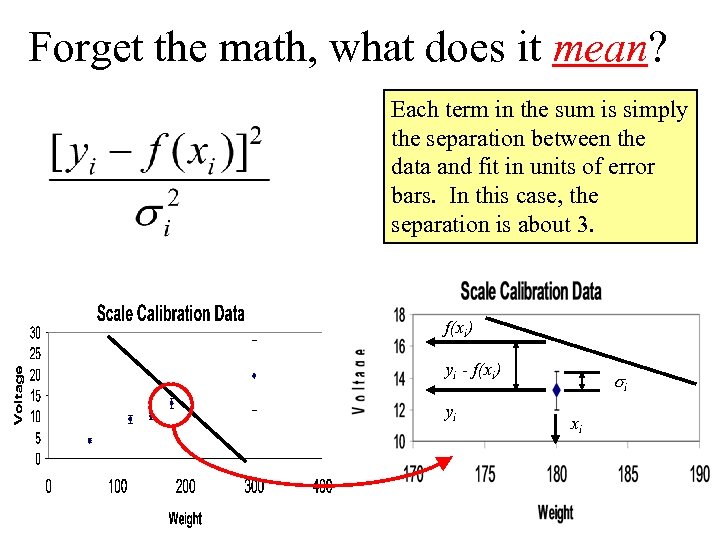Forget the math, what does it mean? Each term in the sum is simply the separation between the data and fit in units of error bars. In this case, the separation is about 3. f(xi) yi - f(xi) yi si xi

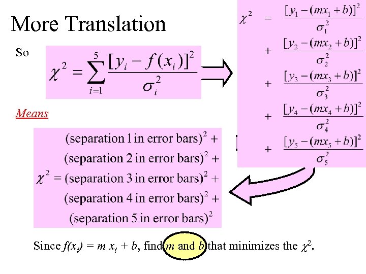More Translation So Means Since f(xi) = m xi + b, find m and b that minimizes the c 2.

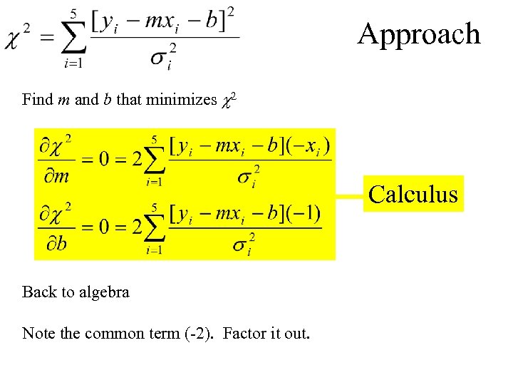Approach Find m and b that minimizes c 2 Calculus Back to algebra Note the common term (-2). Factor it out.

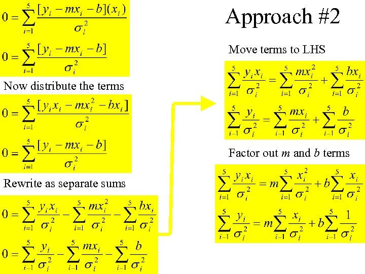Approach #2 Move terms to LHS Now distribute the terms Factor out m and b terms Rewrite as separate sums

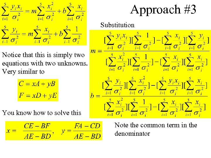Approach #3 Substitution Notice that this is simply two equations with two unknowns. Very similar to You know how to solve this Note the common term in the denominator

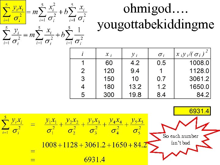ohmigod…. yougottabekiddingme So each number isn’t bad

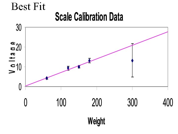
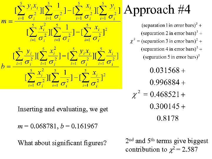Approach #4 Inserting and evaluating, we get m = 0. 068781, b = 0. 161967 What about significant figures? 2 nd and 5 th terms give biggest contribution to c 2 = 2. 587

Best Fit

Best vs. Good Best

Doesn’t always mean good

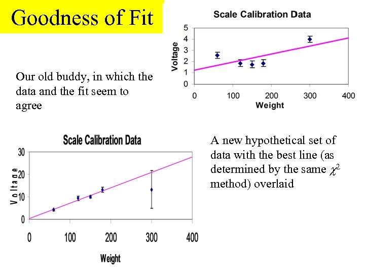Goodness of Fit Our old buddy, in which the data and the fit seem to agree A new hypothetical set of data with the best line (as determined by the same c 2 method) overlaid

New Important Concept • If you have 2 data points and a polynomial of order 1 (line, parameters m & b), then your line will exactly go through your data • If you have 3 data points and a polynomial of order 2 (parabola, parameters A, B & C), then your curve will exactly go through your data • To actually test your fit, you need more data than the curve can naturally accommodate. • This is the so-called degrees of freedom.

Degrees of Freedom (dof ) • The dof of any problem is defined to be the number of data points minus the number of parameters. • In our case, • dof = 5 – 2 = 3 • Need to define the c 2/dof

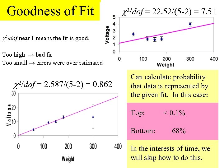Goodness of Fit c 2/dof = 22. 52/(5 -2) = 7. 51 c 2/dof near 1 means the fit is good. Too high bad fit Too small errors were over estimated c 2/dof = 2. 587/(5 -2) = 0. 862 Can calculate probability that data is represented by the given fit. In this case: Top: Bottom: < 0. 1% 68% In the interests of time, we will skip how to do this.

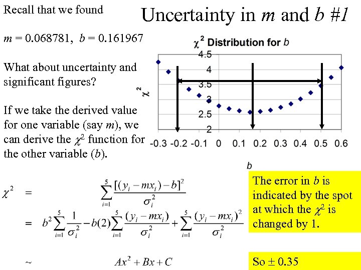Recall that we found Uncertainty in m and b #1 m = 0. 068781, b = 0. 161967 What about uncertainty and significant figures? If we take the derived value for one variable (say m), we can derive the c 2 function for the other variable (b). The error in b is indicated by the spot at which the c 2 is changed by 1. So 0. 35

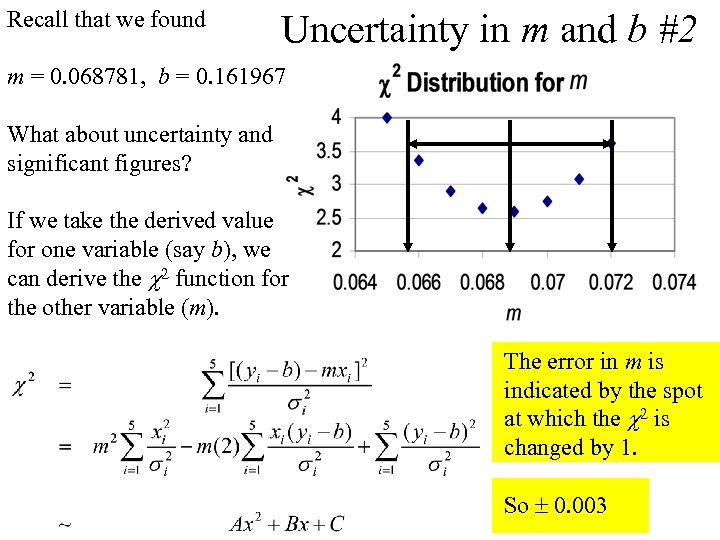Recall that we found Uncertainty in m and b #2 m = 0. 068781, b = 0. 161967 What about uncertainty and significant figures? If we take the derived value for one variable (say b), we can derive the c 2 function for the other variable (m). The error in m is indicated by the spot at which the c 2 is changed by 1. So 0. 003

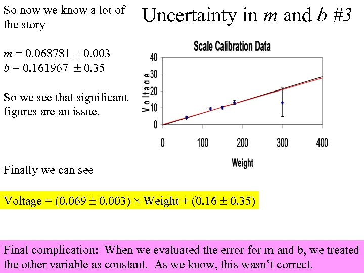So now we know a lot of the story Uncertainty in m and b #3 m = 0. 068781 0. 003 b = 0. 161967 0. 35 So we see that significant figures are an issue. Finally we can see Voltage = (0. 069 0. 003) × Weight + (0. 16 0. 35) Final complication: When we evaluated the error for m and b, we treated the other variable as constant. As we know, this wasn’t correct.

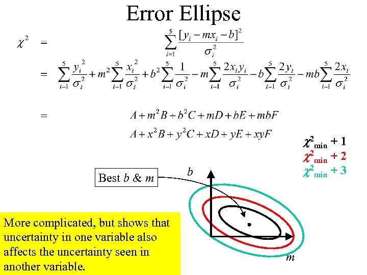Error Ellipse Best b & m More complicated, but shows that uncertainty in one variable also affects the uncertainty seen in another variable. c 2 min + 1 c 2 min + 2 c 2 min + 3 b m

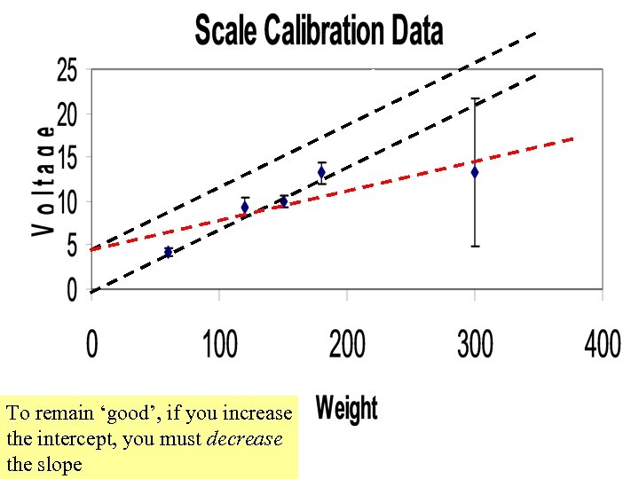e m e sa l , ept c k s ep e r inte se a re Inc To remain ‘good’, if you increase the intercept, you must decrease the slope e th op

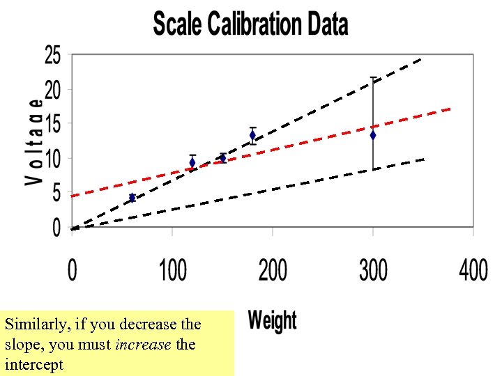e, lop rease s ec D Similarly, if you decrease the slope, you must increase the intercept me t the sa ep p interc kee

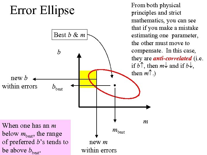From both physical principles and strict mathematics, you can see that if you make a mistake estimating one parameter, the other must move to compensate. In this case, they are anti-correlated (i. e. if b , then m and if b , then m. ) Error Ellipse Best b & m b new b within errors bbest When one has an m below mbest, the range of preferred b’s tends to be above bbest. m mbest new m within errors

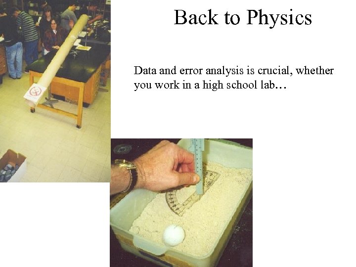Back to Physics Data and error analysis is crucial, whether you work in a high school lab…

Or the Frontier!!!!

References • P. Bevington and D. Robinson, Data Reduction and Error Analysis for the Physical Sciences, 2 nd Edition, Mc. Graw-Hill, Inc. New York, 1992. • J. Taylor, An Introduction to Error Analysis, Oxford University Press, 1982. • Rotated ellipses – http: //www. mecca. org/~halfacre/MATH/rotation. htm

http: //www-d 0. fnal. gov/~lucifer/Power. Point/HSMath. ppt

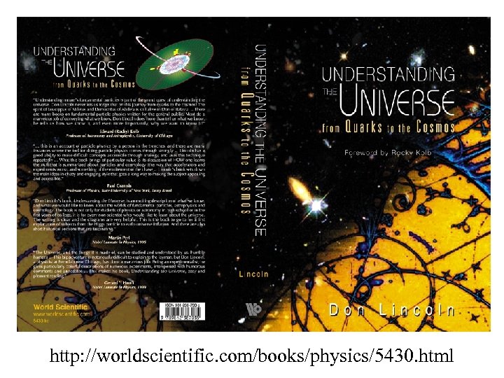http: //worldscientific. com/books/physics/5430. html