High Performance Correlation Techniques For Time Series Xiaojian

High Performance Correlation Techniques For Time Series Xiaojian Zhao Department of Computer Science Courant Institute of Mathematical Sciences New York university 25 Oct. 2004 1

Roadmap Section 1: Introduction Ø Ø Motivation Problem Statement Section 2 : Background Ø Ø Ø GEMINI framework Random Projection Grid Structure Some Definitions Naive method and Yunyue’s Approach Section 3 : Sketch based Stat. Stream Ø Ø Ø Efficient Sketch Computation Sketch technique as a filter Parameter selection Grid structure System Integration Section 4 : Empirical Study Section 5 : Future Work Section 6 : Conclusion 2

Section 1: Introduction 3

Motivation n Stock prices streams n The New York Stock Exchange (NYSE) n 50, 000 securities (streams); 100, 000 ticks (trade and quote) Pairs Trading, a. k. a. Correlation Trading Query: “which pairs of stocks were correlated with a value of over 0. 9 for the last three hours? ” XYZ and ABC have been correlated with a correlation of 0. 95 for the last three hours. Now XYZ and ABC become less correlated as XYZ goes up and ABC goes down. They should converge back later. I will sell XYZ and buy ABC … 4

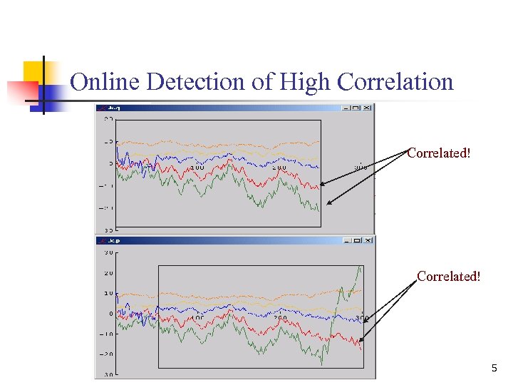Online Detection of High Correlation Correlated! 5

Why speed is important n n n As processors speed up, algorithmic efficiency no longer matters … one might think. True if problem sizes stay same but they don’t. As processors speed up, sensors improve -satellites spewing out a terabyte a day, magnetic resonance imagers give higher resolution images, etc. 6

Problem Statement n n n Detect and report the correlation rapidly and accurately Expand the algorithm into a general engine Apply them in many practical application domains 7

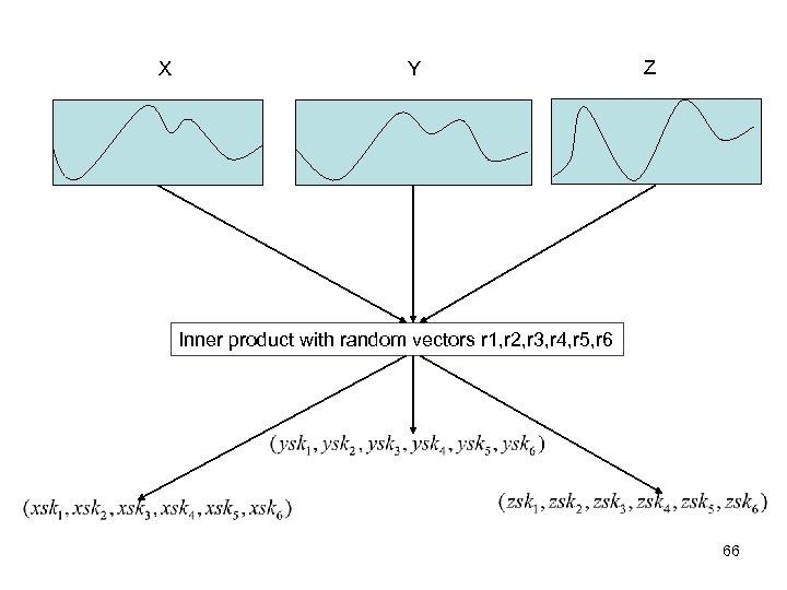
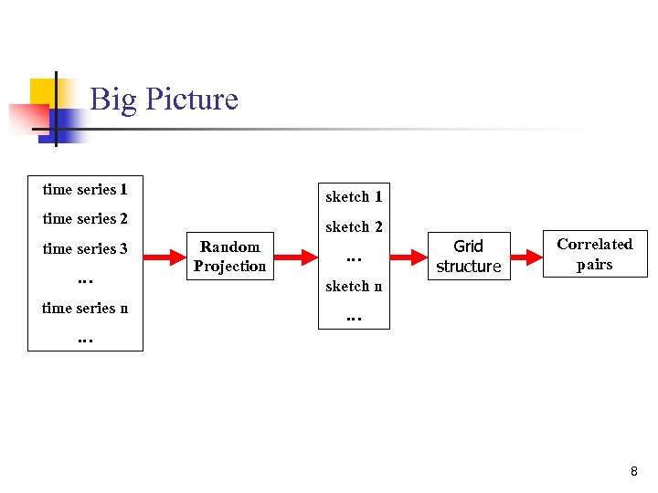Big Picture time series 1 sketch 1 time series 2 sketch 2 time series 3 … time series n Random Projection … Grid structure Correlated pairs sketch n … … 8

Section 2: Background 9

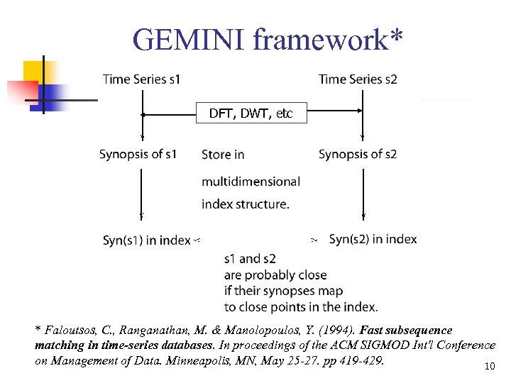GEMINI framework* DFT, DWT, etc * Faloutsos, C. , Ranganathan, M. & Manolopoulos, Y. (1994). Fast subsequence matching in time-series databases. In proceedings of the ACM SIGMOD Int'l Conference on Management of Data. Minneapolis, MN, May 25 -27. pp 419 -429. 10

Goals of GEMINI framework n n High performance Operations on synopses will save time such as distance computation Guarantee no false negative Feature Space shrinks the original distances in the raw data space . 11

Random Projection: Intuition n You are walking in a sparse forest and you are lost. n You have an outdated cell phone without a GPS. n You want to know if you are close to your friend. n n n You identify yourself at 100 meters from the pointy rock and 200 meters from the giant oak etc. If your friend is at similar distances from several of these landmarks, you might be close to one another. The sketches are the set of distances to landmarks. 12

How to make Random Projection* n n n Sketch pool: A list of random vectors drawn from stable distribution (like the landmarks) Project the time series into the space spanned by these random vectors The Euclidean distance (correlation) between time series is approximated by the distance between their sketches with a probabilistic guarantee. • W. B. Johnson and J. Lindenstrauss. “Extensions of Lipshitz mapping into hilbert space”. Contemp. Math. , 26: 189 -206, 1984 13

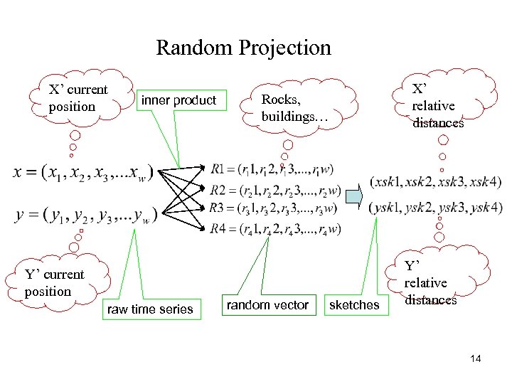Random Projection X’ current position inner product Y’ current position raw time series X’ relative distances Rocks, buildings… random vector sketches Y’ relative distances 14

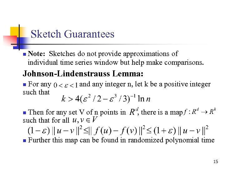Sketch Guarantees n Note: Sketches do not provide approximations of individual time series window but help make comparisons. Johnson-Lindenstrauss Lemma: For any such that n and any integer n, let k be a positive integer Then for any set V of n points in such that for all n n , there is a map Further this map can be found in randomized polynomial time 15

Sketches : Random Projection Why we use sketches or random projections? To reduce the dimensionality! For example: The original time series x is of the length 256, we may represent it with a sketch vector of length 30. First step to removing “the curse of dimensionality” 16

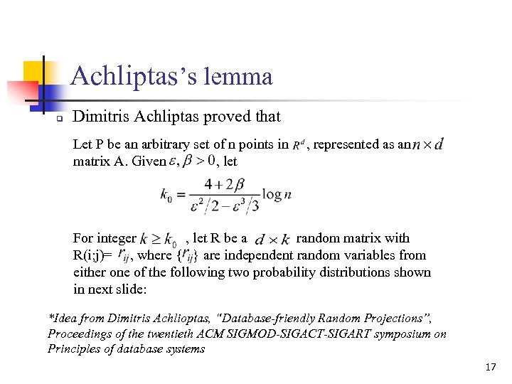Achliptas’s lemma q Dimitris Achliptas proved that Let P be an arbitrary set of n points in matrix A. Given , let , represented as an For integer , let R be a random matrix with R(i; j)= , where { } are independent random variables from either one of the following two probability distributions shown in next slide: *Idea from Dimitris Achlioptas, “Database-friendly Random Projections”, Proceedings of the twentieth ACM SIGMOD-SIGACT-SIGART symposium on Principles of database systems 17

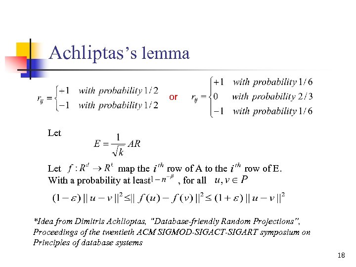Achliptas’s lemma or Let map the With a probability at least row of A to the , for all row of E. *Idea from Dimitris Achlioptas, “Database-friendly Random Projections”, Proceedings of the twentieth ACM SIGMOD-SIGACT-SIGART symposium on Principles of database systems 18

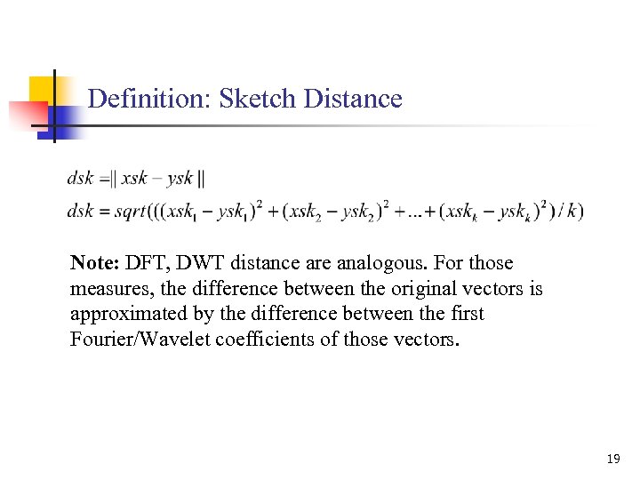Definition: Sketch Distance Note: DFT, DWT distance are analogous. For those measures, the difference between the original vectors is approximated by the difference between the first Fourier/Wavelet coefficients of those vectors. 19

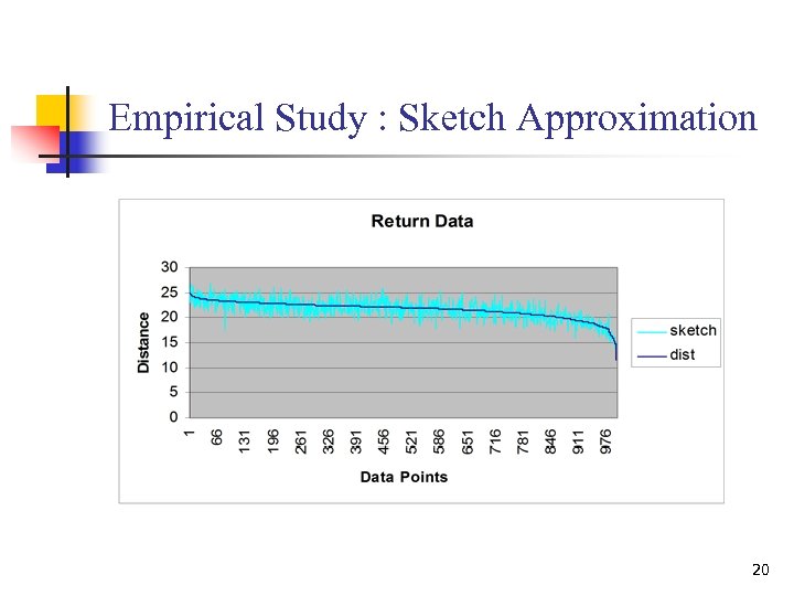Empirical Study : Sketch Approximation 20

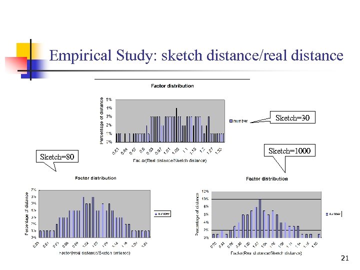Empirical Study: sketch distance/real distance Sketch=30 Sketch=80 Sketch=1000 21

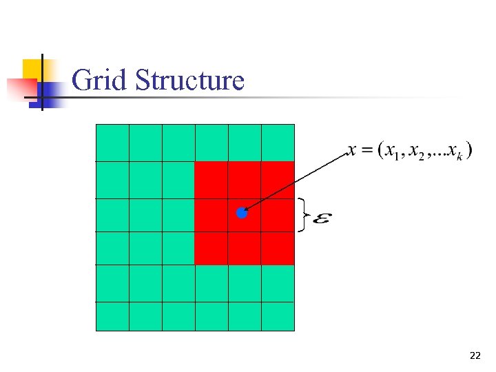Grid Structure 22

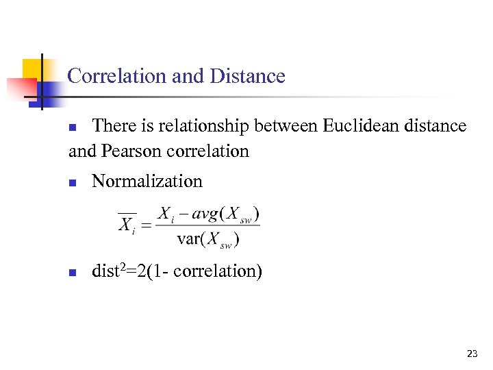Correlation and Distance There is relationship between Euclidean distance and Pearson correlation n n Normalization n dist 2=2(1 - correlation) 23

How to compute the correlation efficiently? Goal: To find the most highly correlated stream pairs over sliding windows n Naive method n Statstream method n Our method 24

Naïve Approach n Space and time cost n n N : number of streams n n Space O(N) and time O(N 2 sw) sw : size of sliding window. Let’s see Statstream approach 25

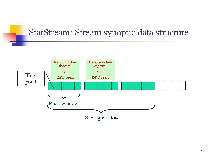
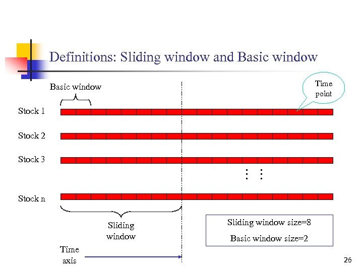Definitions: Sliding window and Basic window Time point Basic window Stock 1 Stock 2 Stock 3 … … Stock n Sliding window Time axis Sliding window size=8 Basic window size=2 26

Stat. Stream Idea n n n Use Discrete Fourier Transform(DFT) to approximate correlation as in the GEMINI approach discussed earlier. Every two minutes (“basic window size”), update the DFT for each time series over the last hour (“sliding window size”) Use a grid structure to filter out unlikely pairs 27

Stat. Stream: Stream synoptic data structure Time point Basic window digests: sum DFT coefs Basic window Sliding window 28

Section 3: Sketch based Stat. Stream 29

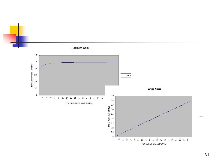
Problem not yet solved n n n DFT approximates the price-like data type very well. Gives a poor approximation for returns (today’s price – yesterday’s price)/yesterday’s price. Return is more like white noise which contains all frequency components. DFT uses the first n (e. g. 10) coefficients in approximating data, which is insufficient in the case of white noise. 30

31

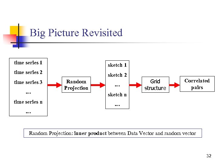Big Picture Revisited time series 1 sketch 1 time series 2 sketch 2 time series 3 … time series n Random Projection … Grid structure Correlated pairs sketch n … … Random Projection: inner product between Data Vector and random vector 32

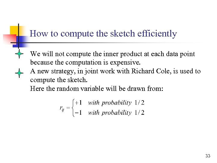How to compute the sketch efficiently We will not compute the inner product at each data point because the computation is expensive. A new strategy, in joint work with Richard Cole, is used to compute the sketch. Here the random variable will be drawn from: 33

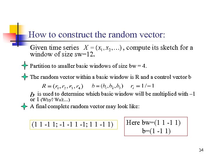How to construct the random vector: Given time series window of size sw=12. , compute its sketch for a Partition to smaller basic windows of size bw = 4. The random vector within a basic window is R and a control vector b is used to determine which basic window will be multiplied with – 1 or 1 (Why? Wait…) A final complete random vector may look like: (1 1 -1 1; -1 -1; 1 1 -1 1) Here bw=(1 1 -1 1) b=(1 -1 1) 34

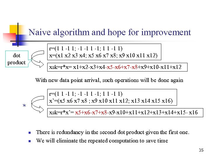Naive algorithm and hope for improvement r=(1 1 -1 1; -1 -1; 1 1 -1 1) x=(x 1 x 2 x 3 x 4; x 5 x 6 x 7 x 8; x 9 x 10 x 11 x 12) dot product xsk=r*x= x 1+x 2 -x 3+x 4 -x 5 -x 6+x 7 -x 8+x 9+x 10 -x 11+x 12 With new data point arrival, such operations will be done again r=(1 1 -1 1; -1 -1; 1 1 -1 1) x’=(x 5 x 6 x 7 x 8 ; x 9 x 10 x 11 x 12; x 13 x 14 x 15 x 16) * xsk=r*x’= x 5+x 6 -x 7+x 8 -x 9 -x 10+x 11+x 12+x 13+x 14+x 15 - x 16 n n There is redundancy in the second dot product given the first one. We will eliminate the repeated computation to save time 35

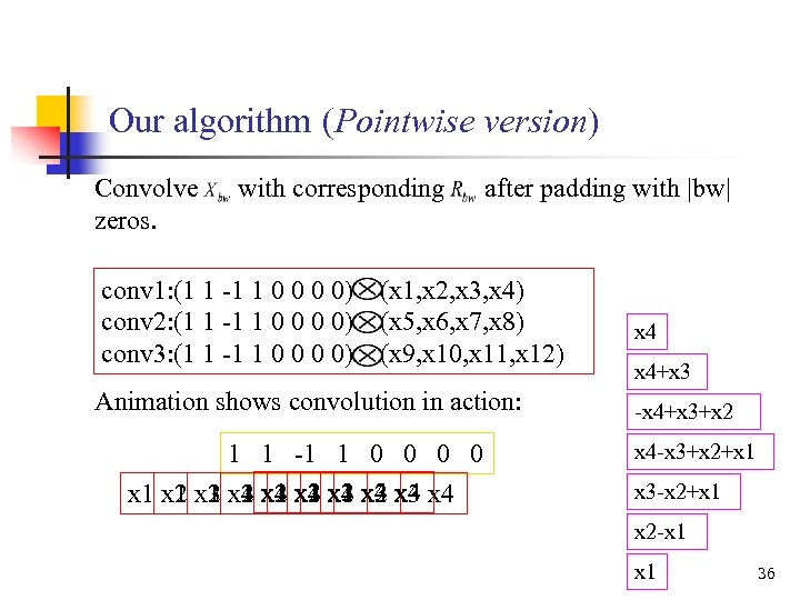Our algorithm (Pointwise version) Convolve zeros. with corresponding conv 1: (1 1 -1 1 0 0) conv 2: (1 1 -1 1 0 0) conv 3: (1 1 -1 1 0 0) after padding with |bw| (x 1, x 2, x 3, x 4) (x 5, x 6, x 7, x 8) (x 9, x 10, x 11, x 12) Animation shows convolution in action: 1 1 -1 1 0 0 x 1 x 2 x 3 x 4 x 4 x 3 x 1 x 2 x 3 x 2 x 1 x 4+x 3 -x 4+x 3+x 2 x 4 -x 3+x 2+x 1 x 3 -x 2+x 1 x 2 -x 1 36

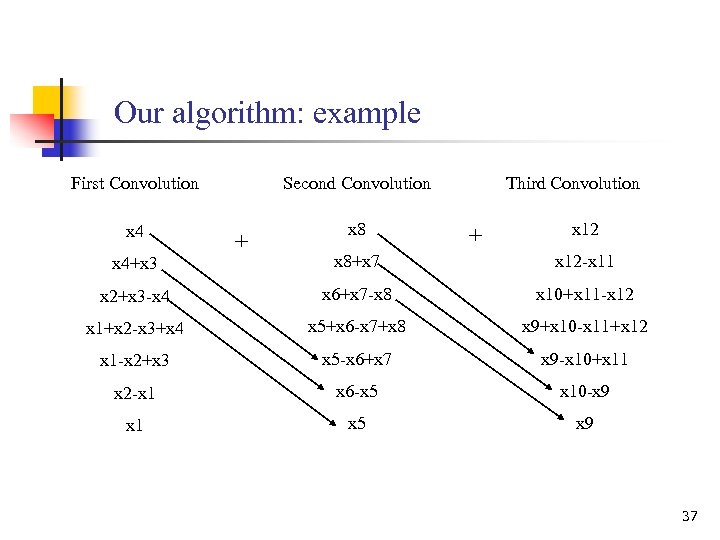Our algorithm: example First Convolution Second Convolution x 4 x 8 + Third Convolution + x 12 x 8+x 7 x 12 -x 11 x 2+x 3 -x 4 x 6+x 7 -x 8 x 10+x 11 -x 12 x 1+x 2 -x 3+x 4 x 5+x 6 -x 7+x 8 x 9+x 10 -x 11+x 12 x 1 -x 2+x 3 x 5 -x 6+x 7 x 9 -x 10+x 11 x 2 -x 1 x 6 -x 5 x 10 -x 9 x 1 x 5 x 9 x 4+x 3 37

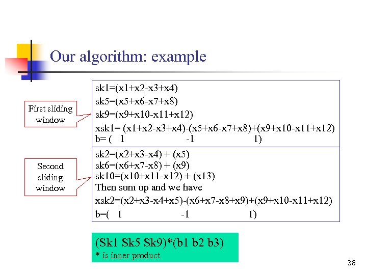Our algorithm: example First sliding window Second sliding window sk 1=(x 1+x 2 -x 3+x 4) sk 5=(x 5+x 6 -x 7+x 8) sk 9=(x 9+x 10 -x 11+x 12) xsk 1= (x 1+x 2 -x 3+x 4)-(x 5+x 6 -x 7+x 8)+(x 9+x 10 -x 11+x 12) b= ( 1 -1 1) sk 2=(x 2+x 3 -x 4) + (x 5) sk 6=(x 6+x 7 -x 8) + (x 9) sk 10=(x 10+x 11 -x 12) + (x 13) Then sum up and we have xsk 2=(x 2+x 3 -x 4+x 5)-(x 6+x 7 -x 8+x 9)+(x 9+x 10 -x 11+x 12) b=( 1 -1 1) (Sk 1 Sk 5 Sk 9)*(b 1 b 2 b 3) * is inner product 38

Our algorithm n n The projection of a sliding window is decomposed into operations over basic windows Each basic window is convolved with each random vector only once We may provide the sketches incrementally starting from each data point. There is no redundancy. 39

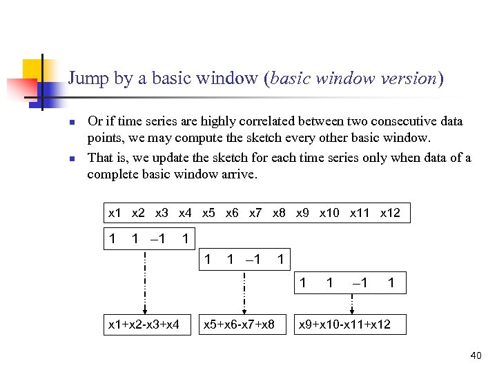Jump by a basic window (basic window version) n n Or if time series are highly correlated between two consecutive data points, we may compute the sketch every other basic window. That is, we update the sketch for each time series only when data of a complete basic window arrive. x 1 x 2 x 3 x 4 x 5 x 6 x 7 x 8 x 9 x 10 x 11 x 12 1 1 – 1 1 1 x 1+x 2 -x 3+x 4 x 5+x 6 -x 7+x 8 1 – 1 1 x 9+x 10 -x 11+x 12 40

Online Version n We take the basic window version for instance Review: To have the same baseline we normalize the time series within each siding window. Challenge: The normalization of the time series change over each basic window 41

Online Version n Its incremental computation nature results in a update of the average and variance whenever a new basic window enters Do we have to compute the normalization and thus the sketch whenever a new basic window enters? Of course not. Otherwise our algorithm will degrade into the trivial computation 42

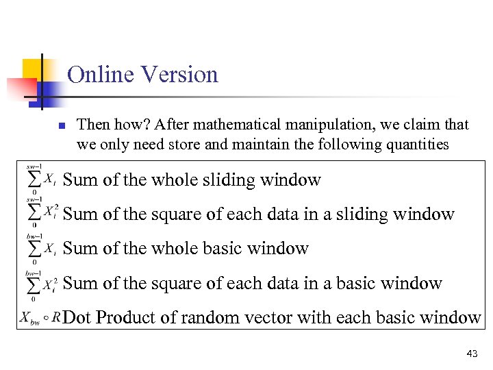Online Version n Then how? After mathematical manipulation, we claim that we only need store and maintain the following quantities Sum of the whole sliding window Sum of the square of each data in a sliding window Sum of the whole basic window Sum of the square of each data in a basic window Dot Product of random vector with each basic window 43

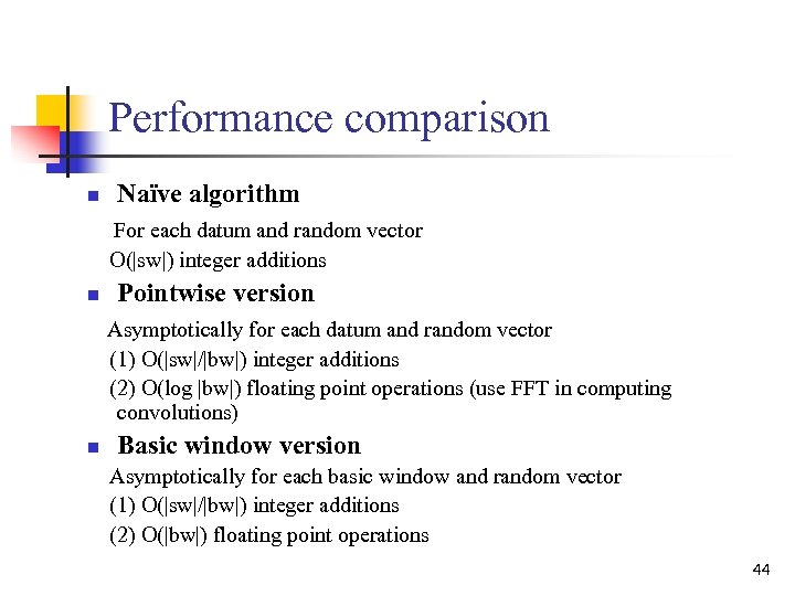Performance comparison n Naïve algorithm For each datum and random vector O(|sw|) integer additions n Pointwise version Asymptotically for each datum and random vector (1) O(|sw|/|bw|) integer additions (2) O(log |bw|) floating point operations (use FFT in computing convolutions) n Basic window version Asymptotically for each basic window and random vector (1) O(|sw|/|bw|) integer additions (2) O(|bw|) floating point operations 44

Sketch distance filter quality n n n We may use the sketch distance to filter the unlikely data pairs How accurate is it? How is it compared to DFT and DWT distance in terms of the approximation ability? 45

Empirical Study: Sketch sketch compared to DFT and DWT distance n n Data length=256 DFT: the first 14 DFT coefficients are used in the distance computation, DWT: db 2 wavelet is used with coefficient size=16 Sketch: the random vector number is 64 46

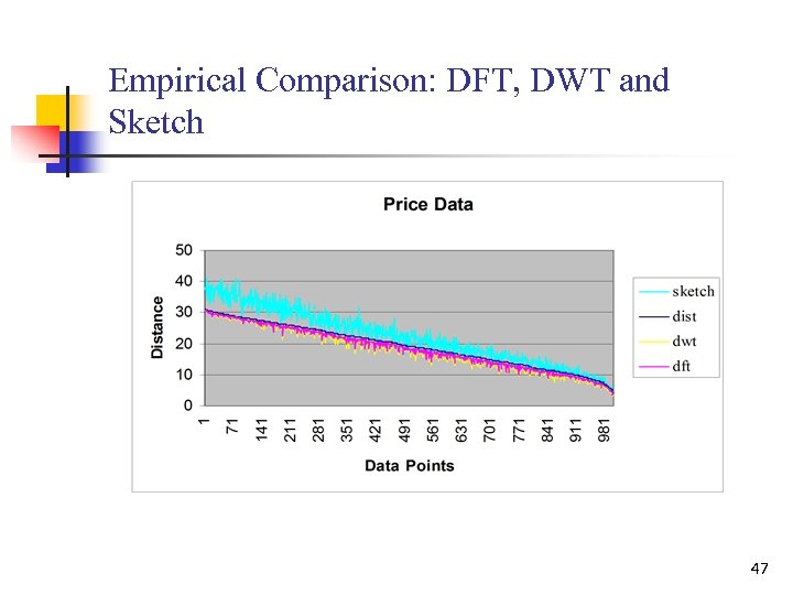Empirical Comparison: DFT, DWT and Sketch 47

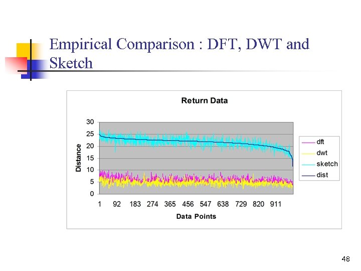Empirical Comparison : DFT, DWT and Sketch 48

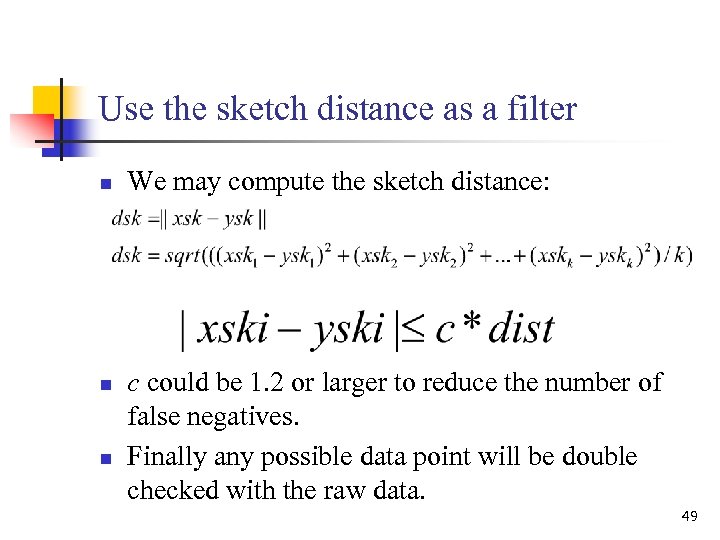Use the sketch distance as a filter n n n We may compute the sketch distance: c could be 1. 2 or larger to reduce the number of false negatives. Finally any possible data point will be double checked with the raw data. 49

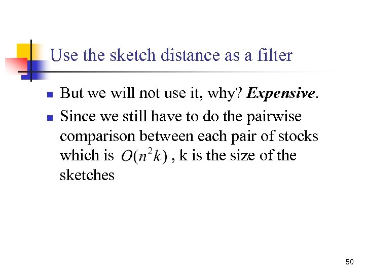Use the sketch distance as a filter n n But we will not use it, why? Expensive. Since we still have to do the pairwise comparison between each pair of stocks which is , k is the size of the sketches 50

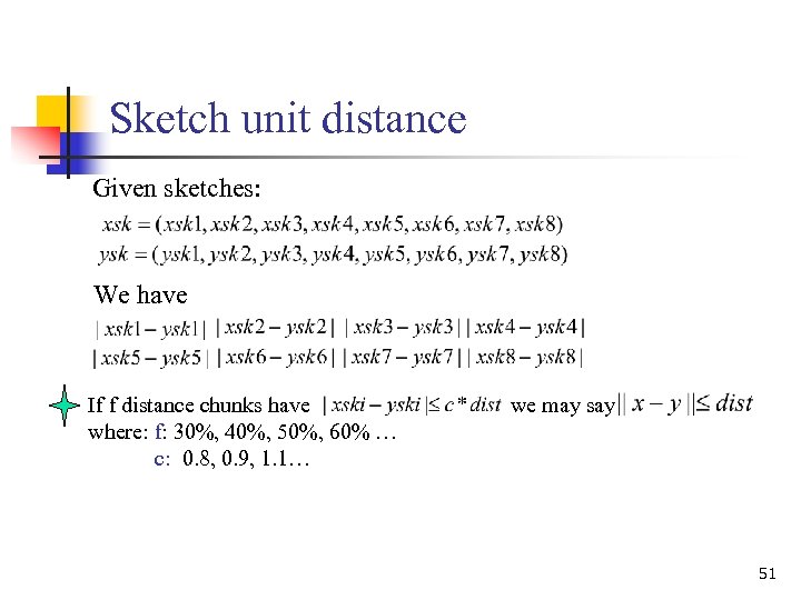Sketch unit distance Given sketches: We have If f distance chunks have where: f: 30%, 40%, 50%, 60% … c: 0. 8, 0. 9, 1. 1… we may say 51

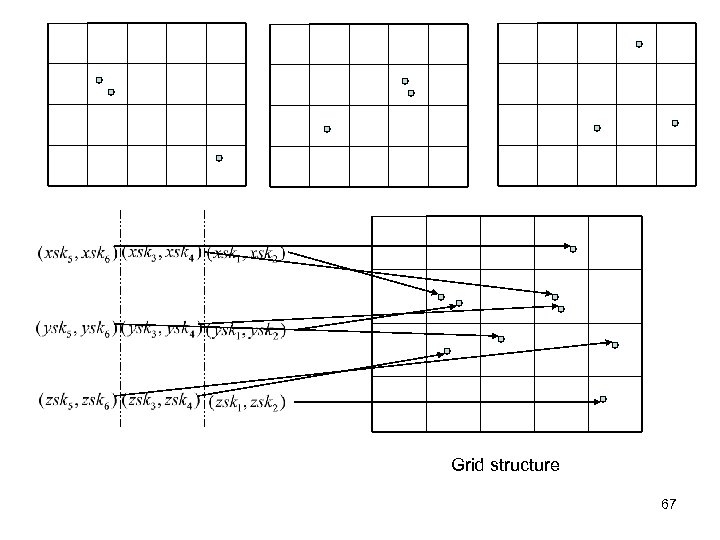
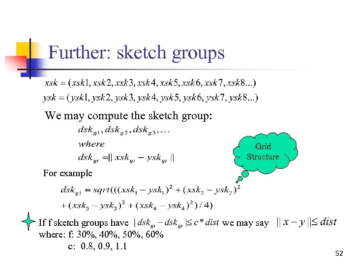Further: sketch groups We may compute the sketch group: Grid Structure For example If f sketch groups have where: f: 30%, 40%, 50%, 60% c: 0. 8, 0. 9, 1. 1 we may say 52

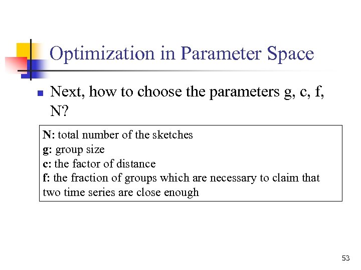Optimization in Parameter Space n Next, how to choose the parameters g, c, f, N? N: total number of the sketches g: group size c: the factor of distance f: the fraction of groups which are necessary to claim that two time series are close enough 53

Optimization in Parameter Space n n Essentially, we will prepare several groups of good parameter candidates and choose the best one to be applied to the practical data But, how to select the good candidates? v Combinatorial Design (CD) v Bootstrapping 54

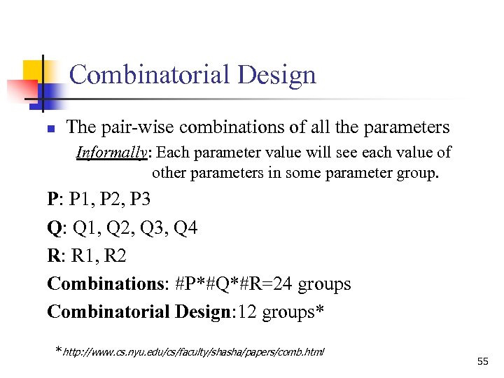Combinatorial Design n The pair-wise combinations of all the parameters Informally: Each parameter value will see each value of other parameters in some parameter group. P: P 1, P 2, P 3 Q: Q 1, Q 2, Q 3, Q 4 R: R 1, R 2 Combinations: #P*#Q*#R=24 groups Combinatorial Design: 12 groups* *http: //www. cs. nyu. edu/cs/faculty/shasha/papers/comb. html 55

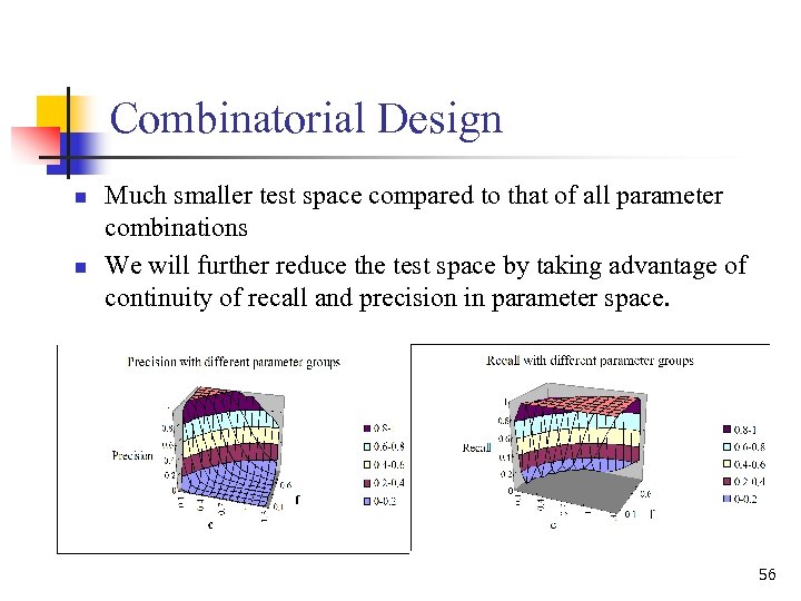Combinatorial Design n n Much smaller test space compared to that of all parameter combinations We will further reduce the test space by taking advantage of continuity of recall and precision in parameter space. 56

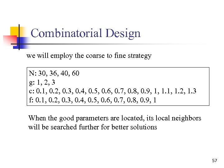Combinatorial Design we will employ the coarse to fine strategy N: 30, 36, 40, 60 g: 1, 2, 3 c: 0. 1, 0. 2, 0. 3, 0. 4, 0. 5, 0. 6, 0. 7, 0. 8, 0. 9, 1, 1. 2, 1. 3 f: 0. 1, 0. 2, 0. 3, 0. 4, 0. 5, 0. 6, 0. 7, 0. 8, 0. 9, 1 When the good parameters are located, its local neighbors will be searched further for better solutions 57

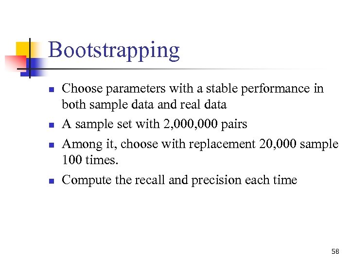Bootstrapping n n Choose parameters with a stable performance in both sample data and real data A sample set with 2, 000 pairs Among it, choose with replacement 20, 000 sample 100 times. Compute the recall and precision each time 58

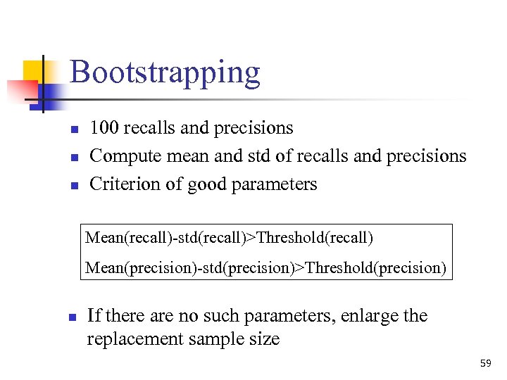Bootstrapping n n n 100 recalls and precisions Compute mean and std of recalls and precisions Criterion of good parameters Mean(recall)-std(recall)>Threshold(recall) Mean(precision)-std(precision)>Threshold(precision) n If there are no such parameters, enlarge the replacement sample size 59

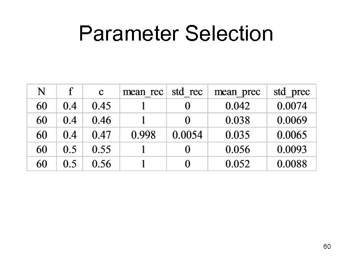Parameter Selection 60

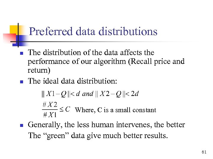Preferred data distributions n n The distribution of the data affects the performance of our algorithm (Recall price and return) The ideal data distribution: Where, C is a small constant n Generally, the less human intervenes, the better The “green” data give much better results. 61

Empirical Study: Various data types v Cstr: Continuous stirred tank reactor v Fortal_ecg: Cutaneous potential recordings of a pregnant woman v Steamgen: Model of a steam generator at Abbott Power Plant in Champaign IL v Winding: Data from a test setup of an industrial winding process v Evaporator: Data from an industrial evaporator v Wind: Daily average wind speeds for 1961 -1978 at 12 synoptic meteorological stations in the Republic of Ireland v Spot_exrates: The spot foreign currency exchange rates v EEG: Electroencepholgram 62

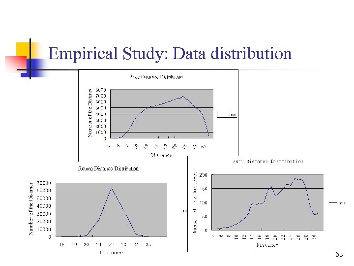Empirical Study: Data distribution 63

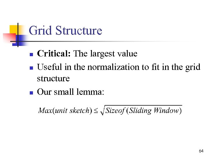Grid Structure n n n Critical: The largest value Useful in the normalization to fit in the grid structure Our small lemma: 64

Grid Structure n n n High correlation => closeness in the vector space To avoid checking all pairs We can use a grid structure and look in the neighborhood, this will return a super set of highly correlated pairs. The data labeled as “potential” will be double checked using the raw data vectors. The pruning power: how many percentage of data are filtered as impossible to be close. 65

X Y Z Inner product with random vectors r 1, r 2, r 3, r 4, r 5, r 6 66

Grid structure 67

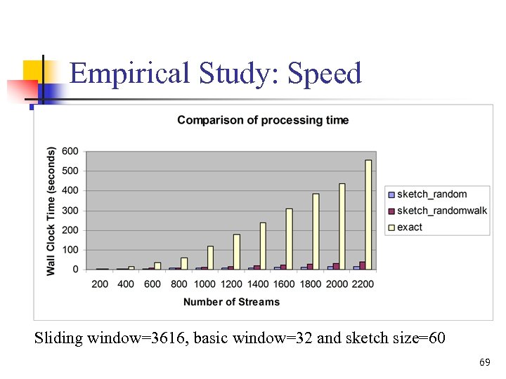
System Integration By combining the sketch scheme with the grid structure, we can § Reduce dimensionality § Eliminate unnecessary pair comparisons The performance can be improved substantially 68

Empirical Study: Speed Sliding window=3616, basic window=32 and sketch size=60 69

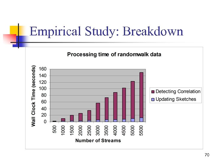Empirical Study: Breakdown 70

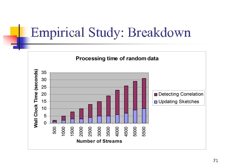Empirical Study: Breakdown 71

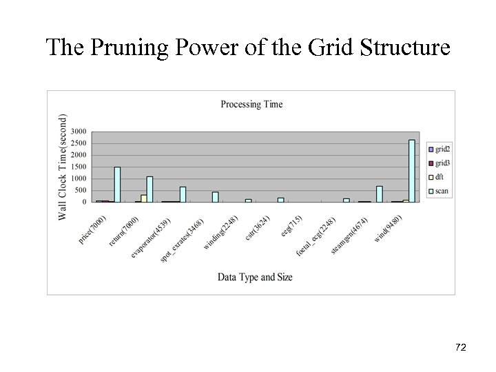The Pruning Power of the Grid Structure 72

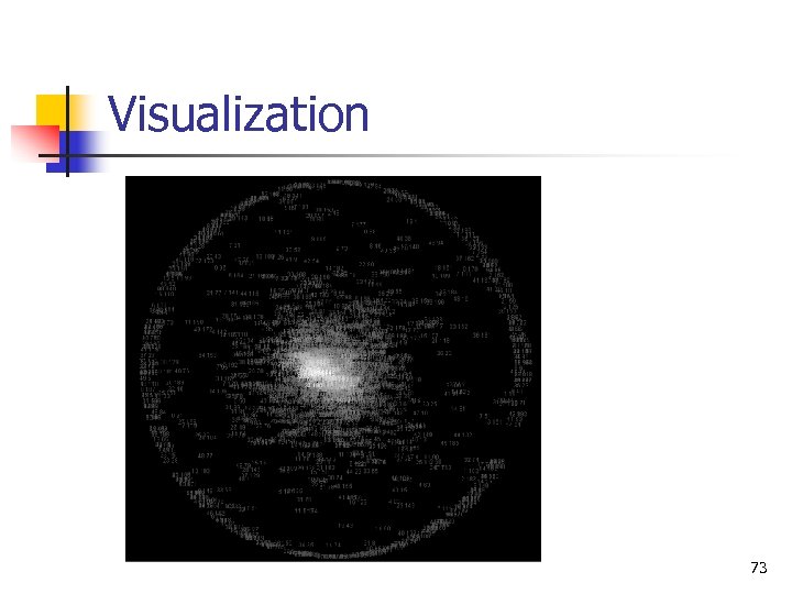Visualization 73

Other applications n n n Cointegration Test Matching Pursuit Anomaly Detection 74

Cointegration Test n n n Make stationary by the linear combination of several non-stationary time series. Model long run characteristic as opposed to the correlation Statstream may be applied to test the stationary condition of cointegration 75

Matching Pursuit n n n Decompose signal into a group of nonorthogonal sub-components Test the correlation among atoms in a dictionary. Expedite the component selection 76

Anomaly Detection n n Measure the relative distance of each point from its nearest neighbors Statstream may serve as a monitor by reporting those points far from any normal points 77

Conclusion n n Introduction GEMINI Framework Random Projection Statstream Review Efficient Sketch Computation Parameter Selection Grid Structure System Integration Empirical Study Future work 78

Thanks a lot! 79

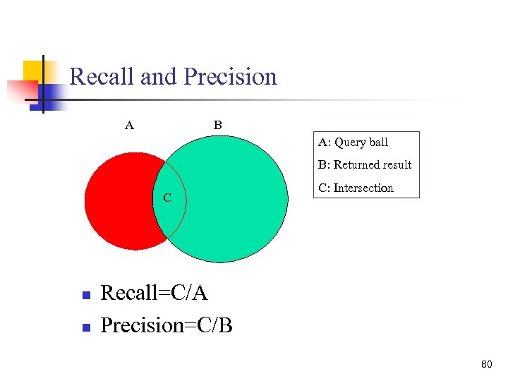Recall and Precision A B A: Query ball B: Returned result C n n C: Intersection Recall=C/A Precision=C/B 80